Overview
The Delta framework answers two related but distinct questions about peptide-level prevalence:
-
Where do peptides shift? —
deltaplot()anddeltaplot_interactive()place each peptide at its pooled prevalence (x) and prevalence shift Δ (y), providing a global view of which features move between groups. -
Is there a statistically significant global shift?
—
compute_delta()aggregates per-peptide z-scores into a single Stouffer-type statistic and assesses significance via subject-label permutation.forestplot()andforestplot_interactive()then display the top and bottom features ranked by that statistic.
This vignette walks through the complete Delta workflow in phiper:
- Visualising raw prevalence shift with
deltaplot()anddeltaplot_interactive() - Running the permutation test with
compute_delta() - Displaying results with
forestplot()andforestplot_interactive()
Setup
Load the bundled example dataset. It contains two patient groups
(A, B) measured at two timepoints
(T1, T2) across 1 000 simulated peptides.
pd <- load_example_data()
#> [09:30:25] INFO  Constructing <phip_data> object
#>                  -> create_data()
#> [09:30:25] INFO  Fetching peptide metadata library via get_peptide_library()
#> [09:30:25] INFO  Retrieving peptide metadata into DuckDB cache
#>                  -> get_peptide_library(force_refresh = FALSE)
#> [09:30:25] INFO  Opened DuckDB connection
#>                    - cache dir:
#>                      /home/runner/.cache/R/phiperio/peptide_meta/phip_cache.duckdb
#>                    - table: peptide_meta
#> [09:30:25] OK    Using cached download (SHA-256 match)
#> [09:30:28] OK    Download complete and loaded into R
#> [09:30:32] INFO  Importing sanitized metadata into DuckDB cache...
#> [09:30:34] OK    peptide_meta table created in DuckDB cache
#> [09:30:34] OK    Retrieving peptide metadata into DuckDB cache - done
#>                  -> elapsed: 9.51s
#> [09:30:34] OK    Peptide metadata acquired
#> [09:30:34] INFO  Validating <phip_data>
#>                  -> validate_phip_data()
#> [09:30:34] INFO  Checking structural requirements (shape & mandatory columns)
#> [09:30:34] INFO  Checking outcome family availability (exist / fold_change /
#>                  raw_counts)
#> [09:30:34] INFO  Checking collisions with reserved names
#>                    - subject_id, sample_id, timepoint, peptide_id, exist,
#>                      fold_change, counts_input, counts_hit
#> [09:30:34] INFO  Ensuring all columns are atomic (no list-cols)
#> [09:30:34] INFO  Checking key uniqueness
#> [09:30:34] INFO  Validating value ranges & types for outcomes
#> [09:30:34] INFO  Assessing sparsity (NA/zero prevalence vs threshold)
#>                    - warn threshold: 50%
#> [09:30:34] INFO  Checking peptide_id coverage against peptide_library
#> [09:30:34] INFO  Checking full grid completeness (peptide * sample)
#> [09:30:35] OK    Validating <phip_data> - done
#>                  -> elapsed: 0.448s
#> [09:30:35] OK    Constructing <phip_data> object - done
#>                  -> elapsed: 9.961s
pd
#> ── <phip_data> ─────────────────────────────────────────────────────────────────
#>
#> counts (first 5 rows):
#> # A tibble: 5 × 9
#>   sample_id subject_id group timepoint peptide_id exist counts_control
#>   <chr>     <chr>      <chr> <chr>     <chr>      <int>          <int>
#> 1 A_T1_1    1          A     T1        10003          1              5
#> 2 A_T1_1    1          A     T1        10017          1             37
#> 3 A_T1_1    1          A     T1        10023          1             11
#> 4 A_T1_1    1          A     T1        10062          1              0
#> 5 B_T1_1    1          B     T1        10087          1              1
#> # ℹ 2 more variables: counts_hits <int>, fold_change <dbl>
#>
#> table size: 78,200 rows x 9 columns
#>
#> peptide library preview (first 5 rows):
#> # A tibble: 5 × 8
#>   peptide_id    Fullname                 species genus family order class common
#>   <chr>         <chr>                    <chr>   <chr> <chr>  <chr> <chr> <chr>
#> 1 agilent_1     Chromodomain-helicase-D… Homo s… Homo  Homin… Prim… Mamm… Human
#> 2 agilent_10    Lipase 2 precursor (Gly… Staphy… Stap… Staph… Baci… Baci… NA
#> 3 agilent_100   cell surface protein pr… Porphy… Porp… Porph… Bact… Bact… NA
#> 4 agilent_1000  Coagulation factor VIII… Homo s… Homo  Homin… Prim… Mamm… Human
#> 5 agilent_10000 transmembrane serine/th… Mycoba… Myco… Mycob… Myco… Acti… NA
#> ... plus 37 more columns
#>
#> library size: 357,190 rows x 45 columns
#>
#> meta flags:
#>   con:            <duckdb_connection>
#>   longitudinal:   TRUE
#>   exist:          TRUE
#>   fold_change:    TRUE
#>   raw_counts:     FALSE
#>   extra_cols:     group, counts_control, counts_hits
#>   peptide_con:    <duckdb_connection>
#>   materialise_table: TRUE
#>   finalizer_env:  <environment>
#>   full_cross:     FALSE
Note. The example data are entirely simulated and have no biological meaning. They exist solely to demonstrate the API.
The Delta plots consume prevalence tables produced by
compute_pop() (see the POP vignette for details). Compute a
group-level prevalence table first:
pop_group <- compute_pop(
  pd,
  rank_cols  = "peptide_id",
  group_cols = "group"
)
#> [09:30:35] INFO  compute_pop
#> [09:30:35] INFO  compute_pop
#>                    - ranks : peptide_id
#>                    - group_cols: group
#>                    - exist_col : exist
#>                    - pop_k_min : 1
#>                    - paired : FALSE
#> [09:30:35] INFO  ranks resolved
#>                    - available: peptide_id
#> [09:30:35] INFO  computing cohort sizes and validating binary group_cols
#> [09:30:35] INFO  computing presence per sample via k-of-n rule
#> [09:30:35] INFO  counting present samples per feature (pop, unpaired)
#> [09:30:35] INFO  building pairwise comparisons
#> [09:30:37] OK    materialized; computing Fisher p-values
#>                    - table: ph_pop_20260714_093035
#> [09:30:38] OK    done (compute_pop, unpaired)
#>                    - rows : 1950
#>                    - ranks : peptide_id
#>                    - k_min : 1
#> [09:30:38] OK    compute_pop - done
#>                  -> elapsed: 2.929s
head(pop_group)
#>         rank feature group_col group1 n1 N1     prop1 percent1 group2 n2 N2
#> 1 peptide_id   10003     group      A 31 38 0.8157895 81.57895      B  0 42
#> 2 peptide_id   10017     group      A  6 38 0.1578947 15.78947      B  0 42
#> 3 peptide_id   10023     group      A 29 38 0.7631579 76.31579      B  0 42
#> 4 peptide_id   10062     group      A 11 38 0.2894737 28.94737      B  0 42
#> 5 peptide_id   10087     group      A  0 38 0.0000000  0.00000      B  8 42
#> 6 peptide_id   10100     group      A  0 38 0.0000000  0.00000      B 10 42
#>       prop2 percent2       ratio delta_ratio        p_raw n_peptides
#> 1 0.0000000  0.00000 68.52631579   33.263158 8.819969e-16          1
#> 2 0.0000000  0.00000 13.26315789    5.631579 9.186952e-03          1
#> 3 0.0000000  0.00000 64.10526316   31.052632 3.123739e-14          1
#> 4 0.0000000  0.00000 24.31578947   11.157895 1.148463e-04          1
#> 5 0.1904762 19.04762  0.06907895   -6.238095 5.758809e-03          1
#> 6 0.2380952 23.80952  0.05526316   -8.047619 1.180799e-03          1
For the unpaired group comparison with compute_delta(),
each subject must appear at most once per group. Because pd
contains two timepoints per subject, restrict to a single timepoint
first:
Visualising prevalence shift
deltaplot() — static ggplot2
deltaplot() plots each peptide at:
-
x-axis — pooled prevalence
(prop1 + prop2) / 2 -
y-axis — prevalence shift
prop2 − prop1
A dashed horizontal line marks Δ = 0. Arrows and labels indicate the
direction of enrichment. A GAM smooth (controlled by
add_smooth) summarises the trend across pooled
prevalence.
The only required input is a data frame containing
group1, group2, prop1, and
prop2 — which is exactly what compute_pop()
returns.
deltaplot(
  pop_group,
  group_pair_values = c("A", "B"),
  group_labels      = c("Group A", "Group B")
)
#> [09:30:38] INFO  Preparing delta prevalence plot.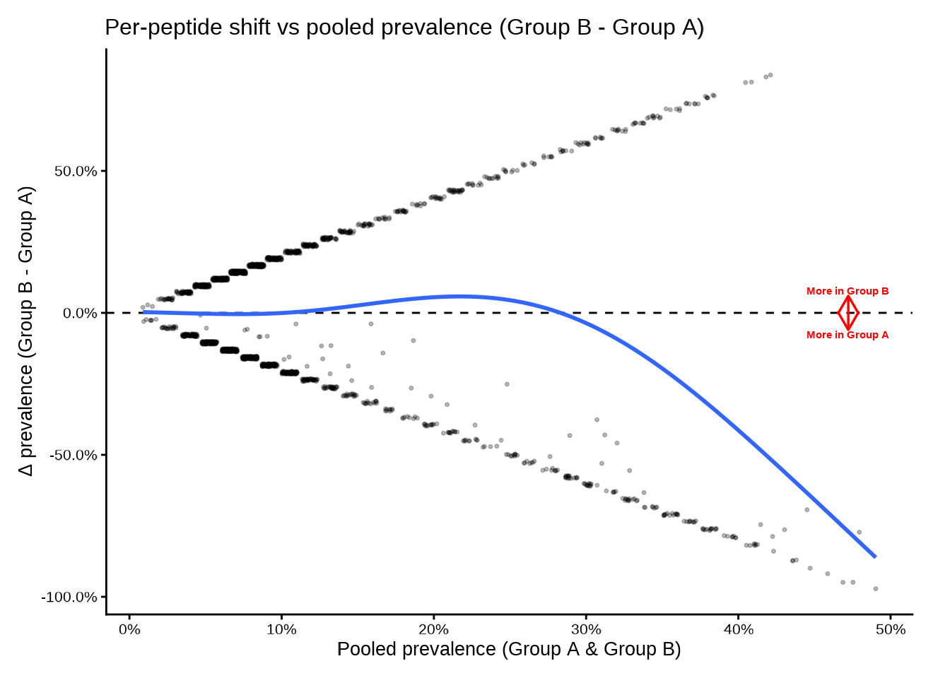
Use group_pair_values to select a specific contrast when
the table contains more than one pair. group_labels
provides display names for the axis annotations.
Adjusting the smooth
The smooth uses a GAM with basis dimension smooth_k.
Lower values produce smoother curves; set
add_smooth = FALSE to suppress it.
deltaplot(
  pop_group,
  group_pair_values  = c("A", "B"),
  group_labels       = c("Group A", "Group B"),
  smooth_k           = 3,
  point_alpha        = 0.15,
  point_size         = 0.4
)
#> [09:30:39] INFO  Preparing delta prevalence plot.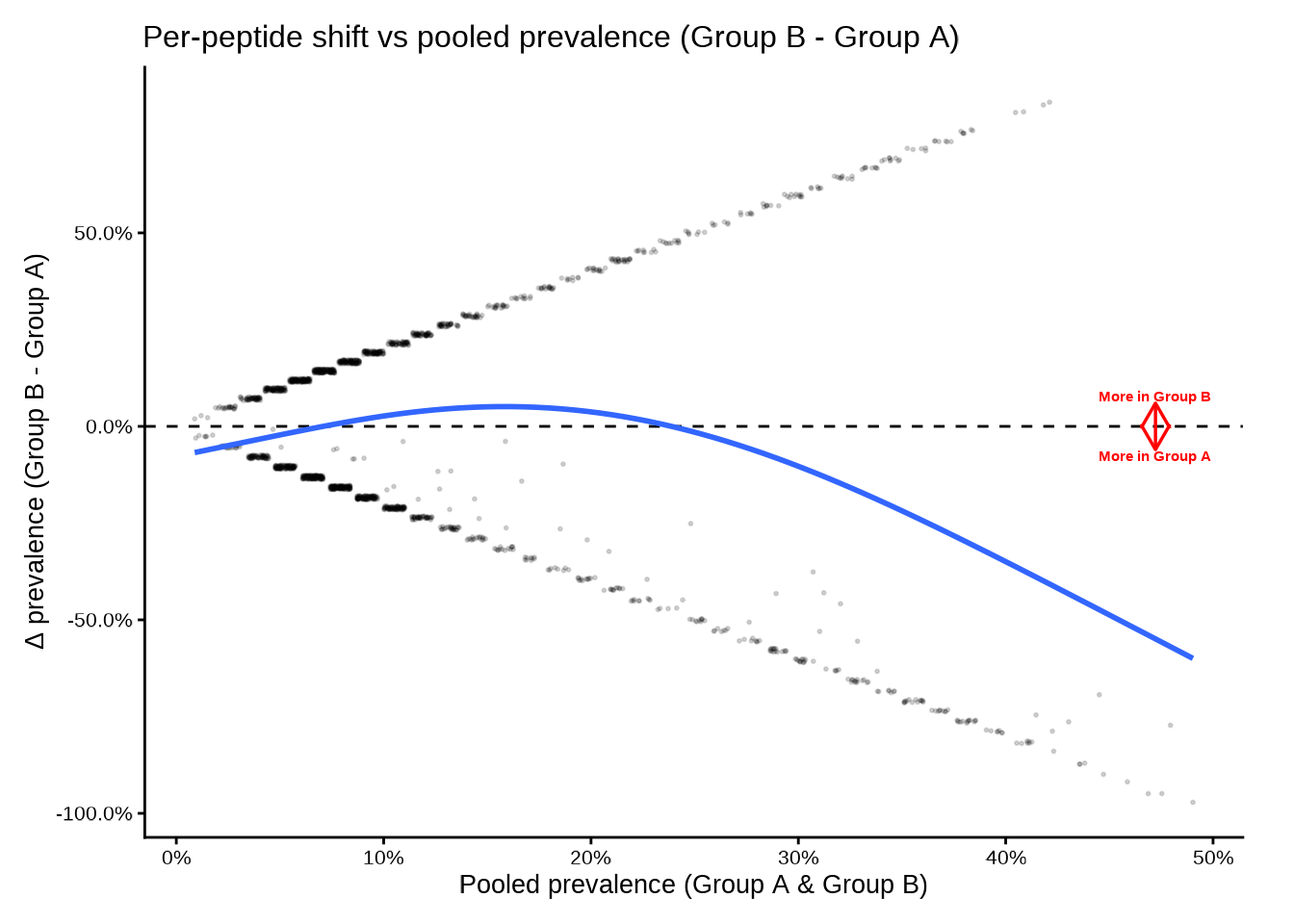
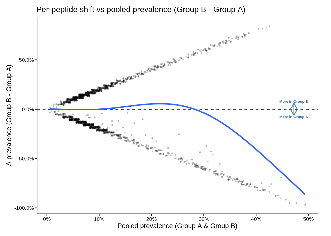
deltaplot_interactive() — plotly
The interactive version mirrors the static API. Hovering over a point shows the feature identifier, group-level counts and percentages, and p-value.
deltaplot_interactive(
  pop_group,
  group_pair_values = c("A", "B"),
  group_labels      = c("Group A", "Group B")
)
Disable the smooth if you have few peptides or want a cleaner display:
deltaplot_interactive(
  pop_group,
  group_pair_values = c("A", "B"),
  group_labels      = c("Group A", "Group B"),
  add_smooth        = FALSE,
  point_size        = 5,
  point_alpha       = 0.5
)
Testing global shift: compute_delta()
compute_delta() performs a permutation test for a global
(antigen-wide) shift in prevalence between two groups. For each
(rank, feature) stratum it computes a per-peptide z-score,
aggregates them via a Stouffer statistic, and assesses significance by
permuting subject labels.
Unpaired design — group comparison
set.seed(42)
delta_group <- compute_delta(
  pd_t1,
  rank_cols      = "peptide_id",
  group_cols     = "group",
  B_permutations = 2000L
)
delta_group
#> # A tibble: 1,950 × 19
#>    rank       feature group_col group1 group2 design   n_subjects_paired
#>    <chr>      <chr>   <chr>     <chr>  <chr>  <chr>                <int>
#>  1 peptide_id 10003   group     A      B      unpaired                NA
#>  2 peptide_id 10017   group     A      B      unpaired                NA
#>  3 peptide_id 10023   group     A      B      unpaired                NA
#>  4 peptide_id 10062   group     A      B      unpaired                NA
#>  5 peptide_id 10087   group     A      B      unpaired                NA
#>  6 peptide_id 10100   group     A      B      unpaired                NA
#>  7 peptide_id 10108   group     A      B      unpaired                NA
#>  8 peptide_id 1011    group     A      B      unpaired                NA
#>  9 peptide_id 10121   group     A      B      unpaired                NA
#> 10 peptide_id 1013    group     A      B      unpaired                NA
#> # ℹ 1,940 more rows
#> # ℹ 12 more variables: n_peptides_used <int>, m_eff <dbl>, T_obs <dbl>,
#> #   T_null_mean <dbl>, T_null_sd <dbl>, T_obs_stand <dbl>, Z_from_p <dbl>,
#> #   p_perm <dbl>, b <int>, max_delta <dbl>, frac_delta_pos <dbl>,
#> #   frac_delta_pos_w <dbl>
What’s in the output?
| Column | Description |
|---|---|
rank |
Rank at which the feature is defined |
feature |
Feature identifier |
group_col |
Name of the grouping column |
group1, group2
|
The two groups compared |
design |
"paired" or "unpaired"
|
n_subjects_paired |
Paired subjects used (or NA for unpaired) |
n_peptides_used |
Peptides contributing to the test |
m_eff |
Effective number of peptides after weighting |
T_obs |
Observed Stouffer-type test statistic |
p_perm |
Two-sided permutation p-value |
b |
Number of permutations actually used |
max_delta |
Maximum absolute peptide-level prevalence difference |
frac_delta_pos |
Unweighted fraction of positive peptide-level deltas |
frac_delta_pos_w |
Weighted fraction of positive peptide-level deltas |
Choosing the per-peptide statistic
stat_mode controls how each peptide’s z-score is
computed:
stat_mode |
Description |
|---|---|
"srlr" (default) |
Signed root likelihood ratio |
"diff" |
Wald-type z: Δ / SE |
"asin" |
Arcsine-transformed z (variance-stabilised) |
"score" |
Pooled score z (2×2 score test) |
"mcnemar" |
Signed McNemar z — paired designs only |
"srlr_paired" |
Signed root deviance — paired designs only |
# Arcsine-transformed statistic
delta_asin <- compute_delta(
  pd,
  rank_cols      = "peptide_id",
  group_cols     = "group",
  stat_mode      = "asin",
  B_permutations = 2000L
)
Aggregation and stratification
aggregate_stat controls how peptide-level z-scores are
combined:
-
"stouffer"(default) — weighted Stouffer combination -
"maxmean"— mean of the dominant direction -
"af"— absolute fraction
strat_bins bins peptides by pooled prevalence before
aggregation. The default bins c(0.002, 0.005, ..., 0.50)
stratify across the prevalence range so that low- and high-prevalence
peptides are treated separately. Set strat_bins = 0 for a
single global statistic without stratification.
# No stratification
delta_nostrat <- compute_delta(
  pd,
  rank_cols      = "peptide_id",
  group_cols     = "group",
  strat_bins     = 0,
  B_permutations = 2000L
)

# Custom bins
delta_custom <- compute_delta(
  pd,
  rank_cols      = "peptide_id",
  group_cols     = "group",
  strat_bins     = c(0.05, 0.25, 0.50),
  B_permutations = 2000L
)
Weighting
weight_mode controls peptide weights in the Stouffer
statistic:
-
"equal"(default) — all peptides weight 1 -
"se_invvar"— inverse-SE weights (downweights noisy peptides) -
"n_eff_sqrt"— square root of expected positives (emphasises common peptides)
delta_invvar <- compute_delta(
  pd,
  rank_cols      = "peptide_id",
  group_cols     = "group",
  weight_mode    = "se_invvar",
  B_permutations = 2000L
)
Paired design — timepoint comparison
When the same subjects are measured at two timepoints, set
paired_by to the subject-linking column and
stat_mode to a paired statistic. The function then performs
sign-flipping permutations instead of label shuffling.
set.seed(42)
delta_paired <- compute_delta(
  pd,
  rank_cols      = "peptide_id",
  group_cols     = "timepoint",
  paired_by      = "subject_id",
  stat_mode      = "srlr_paired",
  B_permutations = 2000L
)
delta_paired
#> # A tibble: 1,946 × 19
#>    rank       feature group_col group1 group2 design n_subjects_paired
#>    <chr>      <chr>   <chr>     <chr>  <chr>  <chr>              <int>
#>  1 peptide_id 10003   timepoint T1     T2     paired                21
#>  2 peptide_id 10017   timepoint T1     T2     paired                21
#>  3 peptide_id 10023   timepoint T1     T2     paired                21
#>  4 peptide_id 10062   timepoint T1     T2     paired                21
#>  5 peptide_id 10087   timepoint T1     T2     paired                21
#>  6 peptide_id 10100   timepoint T1     T2     paired                21
#>  7 peptide_id 10108   timepoint T1     T2     paired                21
#>  8 peptide_id 1011    timepoint T1     T2     paired                21
#>  9 peptide_id 10121   timepoint T1     T2     paired                21
#> 10 peptide_id 1013    timepoint T1     T2     paired                21
#> # ℹ 1,936 more rows
#> # ℹ 12 more variables: n_peptides_used <int>, m_eff <dbl>, T_obs <dbl>,
#> #   T_null_mean <dbl>, T_null_sd <dbl>, T_obs_stand <dbl>, Z_from_p <dbl>,
#> #   p_perm <dbl>, b <int>, max_delta <dbl>, frac_delta_pos <dbl>,
#> #   frac_delta_pos_w <dbl>
Forest plots
Forest plots display the most extreme positive and negative features for a chosen rank, sorted by the selected test statistic.
forestplot() — static ggplot2
forestplot(
  delta_group,
  rank_of_interest  = "peptide_id",
  statistic_to_plot = "T",
  n_neg_each        = 10,
  n_pos_each        = 10,
  left_label        = "More in A",
  right_label       = "More in B"
)$plot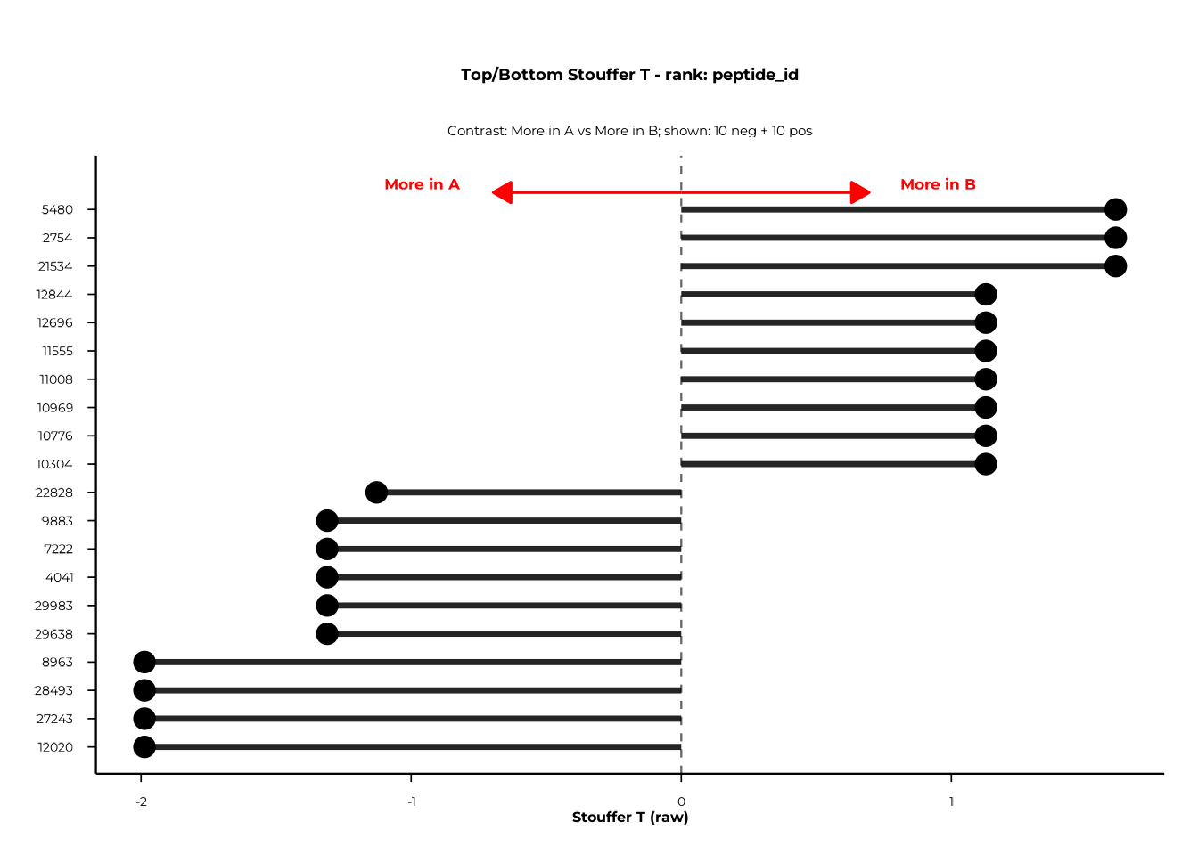
statistic_to_plot selects what is plotted on the
x-axis:
| Value | Description |
|---|---|
"T" |
Raw T_obs from compute_delta()
|
"T_stand" |
Permutation-standardised T (requires T_obs_stand
column) |
"Z_from_p" |
Signed Z derived from permutation p-values (requires
Z_from_p) |
Diverging colours
Set use_diverging_colors = TRUE to shade bars from blue
(negative) to red (positive):
forestplot(
  delta_group,
  rank_of_interest     = "peptide_id",
  statistic_to_plot    = "T",
  n_neg_each           = 10,
  n_pos_each           = 10,
  left_label           = "More in A",
  right_label          = "More in B",
  use_diverging_colors = TRUE
)$plot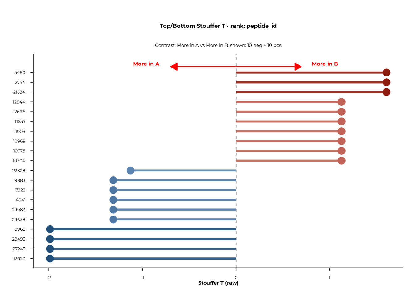
Filtering to significant features
Pass a column name to filter_significant to restrict the
plot to features below a given significance threshold. With
p_perm this retains only permutation-significant
features.
forestplot(
  delta_group,
  rank_of_interest   = "peptide_id",
  statistic_to_plot  = "T",
  filter_significant = "p_perm",
  sig_level          = 0.05,
  left_label         = "More in A",
  right_label        = "More in B"
)$plot
forestplot_interactive() — plotly
The interactive version mirrors the static API and returns a plotly widget. Hovering over a bar shows the feature identifier and statistic value.
forestplot_interactive(
  delta_group,
  rank_of_interest     = "peptide_id",
  statistic_to_plot    = "T",
  n_neg_each           = 10,
  n_pos_each           = 10,
  left_label           = "More in A",
  right_label          = "More in B",
  use_diverging_colors = TRUE
)$plot
Putting it all together
A typical Delta analysis runs in four steps:
# 1. Compute prevalence (needed for deltaplot)
pop <- compute_pop(
  pd,
  rank_cols  = "peptide_id",
  group_cols = "group"
)

# 2. Visualise raw shift
deltaplot(pop, group_pair_values = c("A", "B"),
          group_labels = c("Group A", "Group B"))
deltaplot_interactive(pop, group_pair_values = c("A", "B"),
                      group_labels = c("Group A", "Group B"))

# 3. Permutation test (unpaired)
set.seed(42)
delta <- compute_delta(
  pd,
  rank_cols      = "peptide_id",
  group_cols     = "group",
  B_permutations = 2000L
)

# Optional: paired test across timepoints
delta_paired <- compute_delta(
  pd,
  rank_cols      = "peptide_id",
  group_cols     = "timepoint",
  paired_by      = "subject_id",
  stat_mode      = "srlr_paired",
  B_permutations = 2000L
)

# 4. Forest plots
forestplot(delta, rank_of_interest = "peptide_id",
           left_label = "More in A", right_label = "More in B")$plot
forestplot_interactive(delta, rank_of_interest = "peptide_id",
                       left_label = "More in A",
                       right_label = "More in B")$plot
Session info
sessionInfo()
#> R version 4.6.1 (2026-06-24)
#> Platform: x86_64-pc-linux-gnu
#> Running under: Ubuntu 24.04.4 LTS
#>
#> Matrix products: default
#> BLAS:   /usr/lib/x86_64-linux-gnu/openblas-pthread/libblas.so.3
#> LAPACK: /usr/lib/x86_64-linux-gnu/openblas-pthread/libopenblasp-r0.3.26.so;  LAPACK version 3.12.0
#>
#> locale:
#>  [1] LC_CTYPE=C.UTF-8       LC_NUMERIC=C           LC_TIME=C.UTF-8
#>  [4] LC_COLLATE=C.UTF-8     LC_MONETARY=C.UTF-8    LC_MESSAGES=C.UTF-8
#>  [7] LC_PAPER=C.UTF-8       LC_NAME=C              LC_ADDRESS=C
#> [10] LC_TELEPHONE=C         LC_MEASUREMENT=C.UTF-8 LC_IDENTIFICATION=C
#>
#> time zone: UTC
#> tzcode source: system (glibc)
#>
#> attached base packages:
#> [1] stats     graphics  grDevices utils     datasets  methods   base
#>
#> other attached packages:
#> [1] phiper_0.4.3
#>
#> loaded via a namespace (and not attached):
#>  [1] future_1.70.0         tidyr_1.3.2           utf8_1.2.6
#>  [4] sass_0.4.10           generics_0.1.4        lattice_0.22-9
#>  [7] listenv_1.0.0         digest_0.6.39         magrittr_2.0.5
#> [10] evaluate_1.0.5        grid_4.6.1            RColorBrewer_1.1-3
#> [13] sysfonts_0.8.9        showtextdb_3.0        blob_1.3.0
#> [16] fastmap_1.2.0         Matrix_1.7-5          jsonlite_2.0.0
#> [19] DBI_1.3.0             mgcv_1.9-4            purrr_1.2.2
#> [22] scales_1.4.0          codetools_0.2-20      textshaping_1.0.5
#> [25] jquerylib_0.1.4       duckdb_1.5.4.3        cli_3.6.6
#> [28] rlang_1.3.0           chk_0.10.0            dbplyr_2.6.0
#> [31] phiperio_0.5.2        future.apply_1.20.2   parallelly_1.48.0
#> [34] splines_4.6.1         withr_3.0.3           cachem_1.1.0
#> [37] yaml_2.3.12           otel_0.2.0            parallel_4.6.1
#> [40] tools_4.6.1           dplyr_1.2.1           ggplot2_4.0.3
#> [43] showtext_0.9-8        globals_0.19.1        vctrs_0.7.3
#> [46] R6_2.6.1              lifecycle_1.0.5       fs_2.1.0
#> [49] htmlwidgets_1.6.4     ragg_1.5.2            pkgconfig_2.0.3
#> [52] desc_1.4.3            pkgdown_2.2.1         RcppParallel_5.1.11-2
#> [55] pillar_1.11.1         bslib_0.11.0          gtable_0.3.6
#> [58] glue_1.8.1            Rcpp_1.1.2            systemfonts_1.3.2
#> [61] xfun_0.60             tibble_3.3.1          tidyselect_1.2.1
#> [64] knitr_1.51            farver_2.1.2          nlme_3.1-169
#> [67] htmltools_0.5.9       labeling_0.4.3        rmarkdown_2.31
#> [70] compiler_4.6.1        S7_0.2.2