Overview
Alpha diversity quantifies the within-sample variety of reactive peptides. In PhIP-seq, each sample’s enrichment profile can be characterised by how many unique peptide species are enriched (richness), how evenly that enrichment is distributed (evenness), or how dominated it is by a single peptide (dominance). These properties change across disease conditions, timepoints, and patient subgroups, making alpha diversity a useful summary statistic for exploratory analysis and hypothesis testing.
This vignette walks through the complete alpha diversity workflow in phiper:
- Computing diversity metrics with
compute_alpha() - Visualising distributions with
plot_alpha()andplot_alpha_interactive() - Testing group differences with
compute_alpha_significance() - Summarising statistical results with
plot_alpha_significance()
Setup
Load the bundled example dataset. It contains two patient groups
(A, B) measured at two timepoints
(T1, T2).
pd <- load_example_data()
#> [09:29:34] INFO  Constructing <phip_data> object
#>                  -> create_data()
#> [09:29:34] INFO  Fetching peptide metadata library via get_peptide_library()
#> [09:29:34] INFO  Retrieving peptide metadata into DuckDB cache
#>                  -> get_peptide_library(force_refresh = FALSE)
#> [09:29:34] INFO  Opened DuckDB connection
#>                    - cache dir:
#>                      /home/runner/.cache/R/phiperio/peptide_meta/phip_cache.duckdb
#>                    - table: peptide_meta
#> [09:29:34] OK    Using cached download (SHA-256 match)
#> [09:29:37] OK    Download complete and loaded into R
#> [09:29:42] INFO  Importing sanitized metadata into DuckDB cache...
#> [09:29:43] OK    peptide_meta table created in DuckDB cache
#> [09:29:43] OK    Retrieving peptide metadata into DuckDB cache - done
#>                  -> elapsed: 9.494s
#> [09:29:43] OK    Peptide metadata acquired
#> [09:29:43] INFO  Validating <phip_data>
#>                  -> validate_phip_data()
#> [09:29:43] INFO  Checking structural requirements (shape & mandatory columns)
#> [09:29:44] INFO  Checking outcome family availability (exist / fold_change /
#>                  raw_counts)
#> [09:29:44] INFO  Checking collisions with reserved names
#>                    - subject_id, sample_id, timepoint, peptide_id, exist,
#>                      fold_change, counts_input, counts_hit
#> [09:29:44] INFO  Ensuring all columns are atomic (no list-cols)
#> [09:29:44] INFO  Checking key uniqueness
#> [09:29:44] INFO  Validating value ranges & types for outcomes
#> [09:29:44] INFO  Assessing sparsity (NA/zero prevalence vs threshold)
#>                    - warn threshold: 50%
#> [09:29:44] INFO  Checking peptide_id coverage against peptide_library
#> [09:29:44] INFO  Checking full grid completeness (peptide * sample)
#> [09:29:44] OK    Validating <phip_data> - done
#>                  -> elapsed: 0.445s
#> [09:29:44] OK    Constructing <phip_data> object - done
#>                  -> elapsed: 9.942s
pd
#> ── <phip_data> ─────────────────────────────────────────────────────────────────
#>
#> counts (first 5 rows):
#> # A tibble: 5 × 9
#>   sample_id subject_id group timepoint peptide_id exist counts_control
#>   <chr>     <chr>      <chr> <chr>     <chr>      <int>          <int>
#> 1 A_T1_1    1          A     T1        10003          1              5
#> 2 A_T1_1    1          A     T1        10017          1             37
#> 3 A_T1_1    1          A     T1        10023          1             11
#> 4 A_T1_1    1          A     T1        10062          1              0
#> 5 B_T1_1    1          B     T1        10087          1              1
#> # ℹ 2 more variables: counts_hits <int>, fold_change <dbl>
#>
#> table size: 78,200 rows x 9 columns
#>
#> peptide library preview (first 5 rows):
#> # A tibble: 5 × 8
#>   peptide_id    Fullname                 species genus family order class common
#>   <chr>         <chr>                    <chr>   <chr> <chr>  <chr> <chr> <chr>
#> 1 agilent_1     Chromodomain-helicase-D… Homo s… Homo  Homin… Prim… Mamm… Human
#> 2 agilent_10    Lipase 2 precursor (Gly… Staphy… Stap… Staph… Baci… Baci… NA
#> 3 agilent_100   cell surface protein pr… Porphy… Porp… Porph… Bact… Bact… NA
#> 4 agilent_1000  Coagulation factor VIII… Homo s… Homo  Homin… Prim… Mamm… Human
#> 5 agilent_10000 transmembrane serine/th… Mycoba… Myco… Mycob… Myco… Acti… NA
#> ... plus 37 more columns
#>
#> library size: 357,190 rows x 45 columns
#>
#> meta flags:
#>   con:            <duckdb_connection>
#>   longitudinal:   TRUE
#>   exist:          TRUE
#>   fold_change:    TRUE
#>   raw_counts:     FALSE
#>   extra_cols:     group, counts_control, counts_hits
#>   peptide_con:    <duckdb_connection>
#>   materialise_table: TRUE
#>   finalizer_env:  <environment>
#>   full_cross:     FALSE
Computing alpha diversity
Basic usage: peptide-level diversity by group
The workhorse function is compute_alpha(). At minimum,
supply your <phip_data> object, the grouping
column(s), and the rank(s) at which diversity should be computed.
alpha_group <- compute_alpha(
  pd,
  group_cols = "group",
  ranks      = "peptide_id"
)
#> [09:29:44] INFO  Computing alpha diversity (<phip_data>)
#>                  -> group_cols: 'group'; ranks: 'peptide_id'
#> [09:29:44] OK    Computing alpha diversity (<phip_data>) - done
#>                  -> elapsed: 0.224s
The result is a named list with S3 class
"phip_alpha_diversity". Each element is one data frame —
one per group_col plus, optionally, an interaction
element.
class(alpha_group)
#> [1] "phip_alpha_diversity" "list"
names(alpha_group)
#> [1] "group"
head(alpha_group$group)
#> # A tibble: 6 × 8
#>   rank       sample_id group richness shannon_diversity simpson_diversity
#>   <chr>      <chr>     <chr>    <dbl>             <dbl>             <dbl>
#> 1 peptide_id B_T1_19   B          165              5.11             0.994
#> 2 peptide_id B_T1_20   B          170              5.14             0.994
#> 3 peptide_id B_T2_21   B          302              5.71             0.997
#> 4 peptide_id B_T1_23   B          157              5.06             0.994
#> 5 peptide_id B_T2_4    B          286              5.66             0.997
#> 6 peptide_id B_T2_5    B          283              5.65             0.996
#> # ℹ 2 more variables: pielou_evenness <dbl>, berger_parker_dominance <dbl>
What’s in the output?
Each row is one (sample, rank) pair. The five diversity
columns are:
| Column | Metric | Notes |
|---|---|---|
richness |
Number of enriched peptides | Integer; 0 for empty samples |
shannon_diversity |
Shannon entropy H | Base configurable; NA impossible |
simpson_diversity |
Simpson index (1 − Σp²) | Range [0, 1) |
pielou_evenness |
Pielou’s J = H / ln(S) |
NA when richness ≤ 1 |
berger_parker_dominance |
max(p) |
NA when richness = 0 |
names(alpha_group$group)
#> [1] "rank"                    "sample_id"
#> [3] "group"                   "richness"
#> [5] "shannon_diversity"       "simpson_diversity"
#> [7] "pielou_evenness"         "berger_parker_dominance"
Multiple grouping columns
Pass a character vector to group_cols to get one result
per group variable.
alpha_both <- compute_alpha(
  pd,
  group_cols = c("group", "timepoint"),
  ranks      = "peptide_id"
)
#> [09:29:45] INFO  Computing alpha diversity (<phip_data>)
#>                  -> group_cols: 'group', 'timepoint'; ranks: 'peptide_id'
#> [09:29:45] OK    Computing alpha diversity (<phip_data>) - done
#>                  -> elapsed: 0.38s
names(alpha_both)
#> [1] "group"     "timepoint"
Multiple ranks
Ranks are columns in the peptide library — for example
peptide_id for peptide-level diversity, or
family / genus for taxonomic-level
diversity.
alpha_tax <- compute_alpha(
  pd,
  group_cols = "group",
  ranks      = c("peptide_id", "family", "genus")
)
#> [09:29:45] INFO  Computing alpha diversity (<phip_data>)
#>                  -> group_cols: 'group'; ranks: 'peptide_id', 'family', 'genus'
#> [09:29:45] OK    Computing alpha diversity (<phip_data>) - done
#>                  -> elapsed: 0.443s
# Each element now has rows for all three ranks
dplyr::count(alpha_tax$group, rank)
#> # A tibble: 3 × 2
#>   rank           n
#>   <chr>      <int>
#> 1 family        80
#> 2 genus         80
#> 3 peptide_id    80
Group interactions
Set group_interaction = TRUE to also compute diversity
on the combined group × timepoint label. Set
interaction_only = TRUE to skip per-variable tables and
return only the interaction.
alpha_inter <- compute_alpha(
  pd,
  group_cols        = c("group", "timepoint"),
  ranks             = "peptide_id",
  group_interaction = TRUE
)
#> [09:29:46] INFO  Computing alpha diversity (<phip_data>)
#>                  -> group_cols: 'group', 'timepoint'; ranks: 'peptide_id'
#> [09:29:46] OK    Computing alpha diversity (<phip_data>) - done
#>                  -> elapsed: 0.555s
names(alpha_inter)
#> [1] "group"             "timepoint"         "group * timepoint"

# Returns only the interaction table
alpha_inter_only <- compute_alpha(
  pd,
  group_cols        = c("group", "timepoint"),
  ranks             = "peptide_id",
  group_interaction = TRUE,
  interaction_only  = TRUE
)
#> [09:29:46] INFO  Computing alpha diversity (<phip_data>)
#>                  -> group_cols: 'group', 'timepoint'; ranks: 'peptide_id'
#> [09:29:46] OK    Computing alpha diversity (<phip_data>) - done
#>                  -> elapsed: 0.22s
names(alpha_inter_only)
#> [1] "group * timepoint"
Selecting a metric subset
If you only need richness and Shannon diversity, pass the
metrics argument. This is faster and keeps the output
tidy.
alpha_light <- compute_alpha(
  pd,
  group_cols = "group",
  ranks      = "peptide_id",
  metrics    = c("richness", "shannon")
)
#> [09:29:47] INFO  Computing alpha diversity (<phip_data>)
#>                  -> group_cols: 'group'; ranks: 'peptide_id'
#> [09:29:47] OK    Computing alpha diversity (<phip_data>) - done
#>                  -> elapsed: 0.196s
names(alpha_light$group)
#> [1] "rank"              "sample_id"         "group"
#> [4] "richness"          "shannon_diversity"
Shannon base
By default, Shannon diversity is computed in natural log (nats). Use
shannon_base = "log2" (bits) or "log10"
(hartleys) for comparability with other tools.
alpha_ln   <- compute_alpha(pd, group_cols = "group", ranks = "peptide_id",
                             metrics = "shannon", shannon_base = "ln")
#> [09:29:47] INFO  Computing alpha diversity (<phip_data>)
#>                  -> group_cols: 'group'; ranks: 'peptide_id'
#> [09:29:47] OK    Computing alpha diversity (<phip_data>) - done
#>                  -> elapsed: 0.161s
alpha_log2 <- compute_alpha(pd, group_cols = "group", ranks = "peptide_id",
                             metrics = "shannon", shannon_base = "log2")
#> [09:29:47] INFO  Computing alpha diversity (<phip_data>)
#>                  -> group_cols: 'group'; ranks: 'peptide_id'
#> [09:29:47] OK    Computing alpha diversity (<phip_data>) - done
#>                  -> elapsed: 0.159s

# log2 values are ln values divided by ln(2)
head(alpha_ln$group$shannon_diversity / log(2) - alpha_log2$group$shannon_diversity, 3)
#> [1] 0.347923303 0.297968196 0.009522774
Presence modes
mode controls what n represents in every
diversity formula:
| Mode | Rule | Required argument |
|---|---|---|
"binary" (default) |
exist > 0 |
— |
"threshold" |
abundance_col > threshold |
threshold |
"abundance" |
raw abundance_col value |
abundance_col |
mode = "binary" (default)
Binary mode uses the pre-computed exist flag. A peptide
counts as present whenever exist > 0.
alpha_bin <- compute_alpha(
  pd,
  group_cols = "group",
  ranks      = "peptide_id",
  mode       = "binary",
  metrics    = "richness"
)
#> [09:29:47] INFO  Computing alpha diversity (<phip_data>)
#>                  -> group_cols: 'group'; ranks: 'peptide_id'
#> [09:29:48] OK    Computing alpha diversity (<phip_data>) - done
#>                  -> elapsed: 0.163s
summary(alpha_bin$group$richness)
#>    Min. 1st Qu.  Median    Mean 3rd Qu.    Max.
#>   141.0   173.2   201.0   233.8   304.2   339.0
mode = "threshold"
Threshold mode re-defines “present” using a continuous abundance
column (fold_change by default). Only peptides whose
fold-change exceeds threshold are counted. Raising the
threshold sharpens the definition of a “hit” and typically reduces
richness.
# Loose threshold: fold_change > 10
alpha_thr10 <- compute_alpha(
  pd,
  group_cols = "group",
  ranks      = "peptide_id",
  mode       = "threshold",
  threshold  = 10,
  metrics    = "richness"
)
#> [09:29:48] INFO  Computing alpha diversity (<phip_data>)
#>                  -> group_cols: 'group'; ranks: 'peptide_id'
#> [09:29:48] OK    Computing alpha diversity (<phip_data>) - done
#>                  -> elapsed: 0.219s

# Strict threshold: fold_change > 100
alpha_thr100 <- compute_alpha(
  pd,
  group_cols = "group",
  ranks      = "peptide_id",
  mode       = "threshold",
  threshold  = 100,
  metrics    = "richness"
)
#> [09:29:48] INFO  Computing alpha diversity (<phip_data>)
#>                  -> group_cols: 'group'; ranks: 'peptide_id'
#> [09:29:48] OK    Computing alpha diversity (<phip_data>) - done
#>                  -> elapsed: 0.21s

# Richness drops as the threshold increases
data.frame(
  mode      = c("binary", "threshold > 10", "threshold > 100"),
  mean_richness = c(
    mean(alpha_bin$group$richness),
    mean(alpha_thr10$group$richness),
    mean(alpha_thr100$group$richness)
  )
)
#>              mode mean_richness
#> 1          binary      233.8375
#> 2  threshold > 10      949.6750
#> 3 threshold > 100      676.3750
Supply abundance_col to use a different column than
fold_change:
alpha_thr_counts <- compute_alpha(
  pd,
  group_cols    = "group",
  ranks         = "peptide_id",
  mode          = "threshold",
  abundance_col = "counts_hits",
  threshold     = 50
)
mode = "abundance"
Abundance mode does not binarise. Instead, n for each
peptide is its raw value in abundance_col. Diversity
metrics are computed from these continuous weights, making richness
equivalent to the count of peptides with non-zero abundance and Shannon
diversity a weighted entropy.
Tip. Abundance mode operates on a local data frame rather than a DuckDB-backed table. Collect the relevant columns first with
dplyr::collect()before passing them tocompute_alpha().
# Collect the long table to a local data frame
dl <- dplyr::collect(pd$data_long)

alpha_abund <- compute_alpha(
  dl,
  group_cols    = "group",
  ranks         = "peptide_id",
  mode          = "abundance",
  abundance_col = "fold_change",
  metrics       = c("richness", "shannon", "simpson")
)
#> [09:29:48] INFO  Computing alpha diversity (data.frame)
#>                  -> group_cols: 'group'; ranks: 'peptide_id'
#> [09:29:50] OK    Computing alpha diversity (data.frame) - done
#>                  -> elapsed: 1.988s
head(alpha_abund$group[, c("sample_id", "group", "richness",
                            "shannon_diversity", "simpson_diversity")])
#> # A tibble: 6 × 5
#>   sample_id group richness shannon_diversity simpson_diversity
#>   <chr>     <chr>    <dbl>             <dbl>             <dbl>
#> 1 A_T1_1    A         1000              5.83             0.994
#> 2 B_T1_1    B          950              5.78             0.992
#> 3 A_T2_1    A         1000              5.78             0.993
#> 4 B_T2_1    B          950              5.79             0.993
#> 5 A_T1_10   A         1000              5.75             0.993
#> 6 B_T1_10   B          950              5.73             0.992
Compare mean Shannon diversity under binary vs. abundance mode: the abundance-weighted version is typically lower because a few dominant peptides drive the distribution.
data.frame(
  mode          = c("binary", "abundance (fold_change)"),
  mean_shannon  = c(
    mean(alpha_bin$group$shannon_diversity),
    mean(alpha_abund$group$shannon_diversity)
  )
)
#>                      mode mean_shannon
#> 1                  binary           NA
#> 2 abundance (fold_change)     5.796632
When aggregating to a higher rank (e.g. family),
abundance_agg controls how peptide-level values are reduced
within each rank category:
# Sum fold-changes across all peptides per family (collected data frame)
alpha_abund_fam <- compute_alpha(
  dl,
  group_cols    = "group",
  ranks         = "family",
  mode          = "abundance",
  abundance_col = "fold_change",
  abundance_agg = "sum"   # or "mean" (default) or "max"
)
Accessing result attributes
Metadata about the computation is stored as attributes.
attr(alpha_group, "ranks")
#> [1] "peptide_id"
attr(alpha_group, "mode")
#> [1] "binary"
attr(alpha_group, "metrics")
#> [1] "richness"        "shannon"         "simpson"         "pielou_evenness"
#> [5] "berger_parker"
attr(alpha_group, "n_samples")
#> [1] 80
Visualising alpha diversity
plot_alpha() — static boxplots
Pass the result of compute_alpha() to
plot_alpha(). The minimum required argument beyond
x is the name of the metric to plot.
plot_alpha(
  alpha_group,
  metric    = "richness",
  group_col = "group"
)
#> [09:29:50] INFO  plotting alpha diversity (precomputed)
#>                  -> metric: richness
#> [09:29:51] OK    plotting alpha diversity (precomputed) - done
#>                  -> elapsed: 0.091s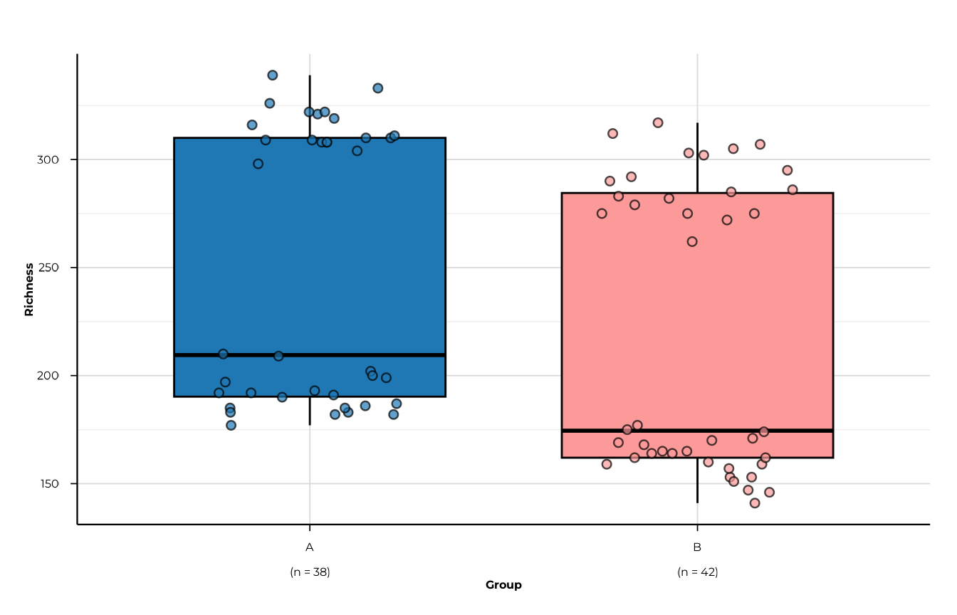
All five metrics
for (m in c("richness", "shannon_diversity", "simpson_diversity",
            "pielou_evenness", "berger_parker_dominance")) {
  print(plot_alpha(alpha_group, metric = m, group_col = "group"))
}
#> [09:29:51] INFO  plotting alpha diversity (precomputed)
#>                  -> metric: richness
#> [09:29:51] OK    plotting alpha diversity (precomputed) - done
#>                  -> elapsed: 0.096s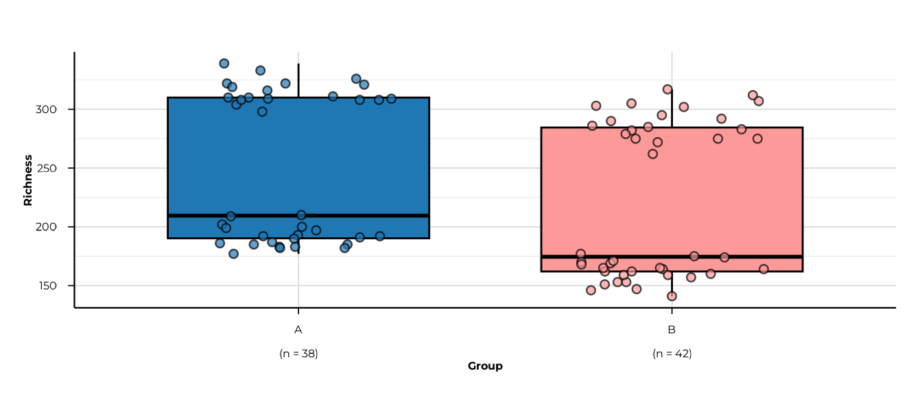
#> [09:29:51] INFO  plotting alpha diversity (precomputed)
#>                  -> metric: shannon_diversity
#> [09:29:51] OK    plotting alpha diversity (precomputed) - done
#>                  -> elapsed: 0.097s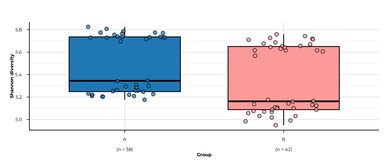
#> [09:29:52] INFO  plotting alpha diversity (precomputed)
#>                  -> metric: simpson_diversity
#> [09:29:52] OK    plotting alpha diversity (precomputed) - done
#>                  -> elapsed: 0.06s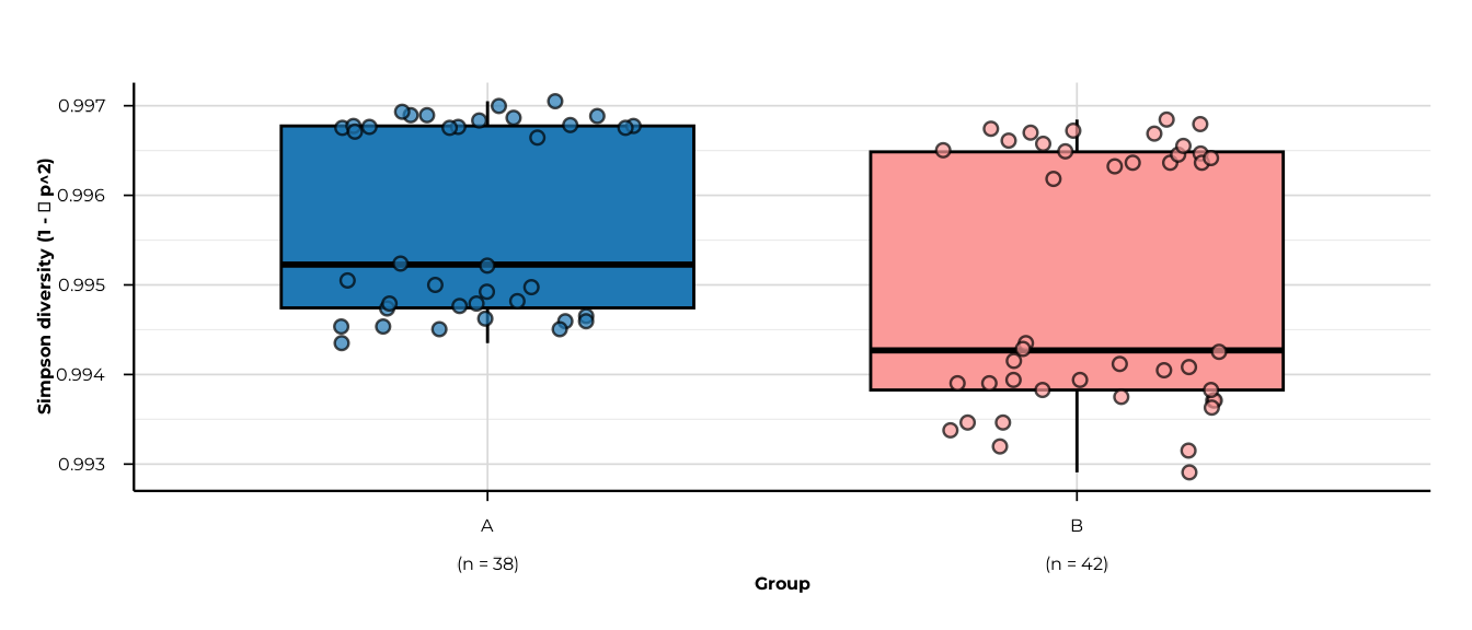
#> [09:29:52] INFO  plotting alpha diversity (precomputed)
#>                  -> metric: pielou_evenness
#> [09:29:52] OK    plotting alpha diversity (precomputed) - done
#>                  -> elapsed: 0.096s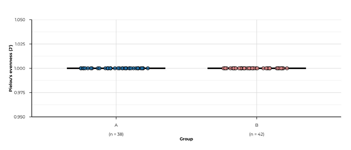
#> [09:29:52] INFO  plotting alpha diversity (precomputed)
#>                  -> metric: berger_parker_dominance
#> [09:29:52] OK    plotting alpha diversity (precomputed) - done
#>                  -> elapsed: 0.06s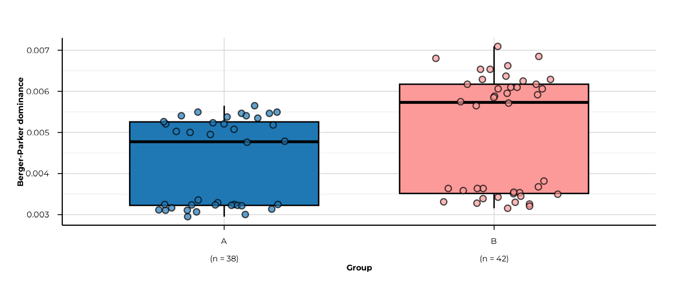
Faceting across multiple ranks
When diversity was computed at multiple ranks, set
facet_by_rank = TRUE (the default) to get one panel per
rank.
Note on this toy example. The peptides shipped with
load_example_data()are synthetic identifiers that do not map to any entry in the peptide library. As a result, all taxonomic rank columns (family,genus, …) are empty for every peptide, so richness at those ranks is 0 for all samples. In a real PhIP-seq experiment where peptides carry proper library annotations, each rank would show non-zero diversity reflecting the taxonomic breadth of each patient’s reactivity.
plot_alpha(
  alpha_tax,
  metric        = "richness",
  group_col     = "group",
  facet_by_rank = TRUE,
  ncol          = 3
)
#> [09:29:53] INFO  plotting alpha diversity (precomputed)
#>                  -> metric: richness
#> [09:29:53] OK    plotting alpha diversity (precomputed) - done
#>                  -> elapsed: 0.102s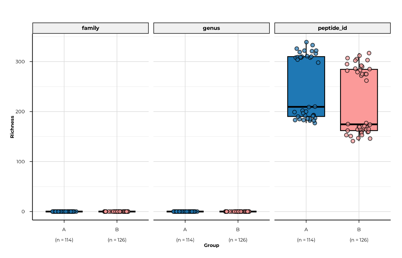
Disable faceting and restrict to a single rank with
filter_ranks.
plot_alpha(
  alpha_tax,
  metric        = "richness",
  group_col     = "group",
  filter_ranks  = "peptide_id",
  facet_by_rank = FALSE
)
#> [09:29:54] INFO  plotting alpha diversity (precomputed)
#>                  -> metric: richness
#> [09:29:54] OK    plotting alpha diversity (precomputed) - done
#> -> elapsed: 0.062s![]()
Filtering and ordering groups
Use filter_groups to keep a subset and
x_order to control axis order.
plot_alpha(
  alpha_both$timepoint,
  metric        = "shannon_diversity",
  group_col     = "timepoint",
  filter_groups = c("T1", "T2"),
  x_order       = c("T1", "T2"),
  x_labels      = c(T1 = "Baseline", T2 = "Follow-up")
)
#> [09:29:54] INFO  plotting alpha diversity (precomputed)
#>                  -> metric: shannon_diversity
#> [09:29:54] OK    plotting alpha diversity (precomputed) - done
#>                  -> elapsed: 0.069s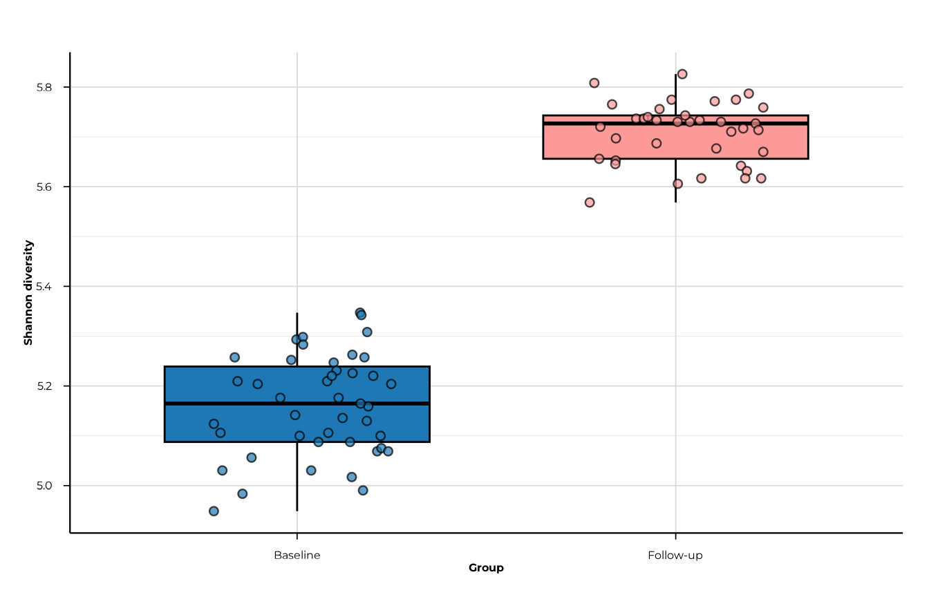
Customising appearance
Simpson diversity values in this dataset are tightly clustered near 1
(range 0.993–0.997). Setting y_range to the actual data
range rather than the theoretical c(0, 1) reveals the
within-group spread that would otherwise be invisible.
plot_alpha(
  alpha_group,
  metric        = "simpson_diversity",
  group_col     = "group",
  custom_colors = c(A = "#E41A1C", B = "#377EB8"),
  y_range       = c(0.99, 1),
  x_tickangle   = 30,
  show_grids    = FALSE,
  point_size    = 2.5,
  point_alpha   = 0.6
)
#> [09:29:55] INFO  plotting alpha diversity (precomputed)
#>                  -> metric: simpson_diversity
#> [09:29:55] OK    plotting alpha diversity (precomputed) - done
#>                  -> elapsed: 0.062s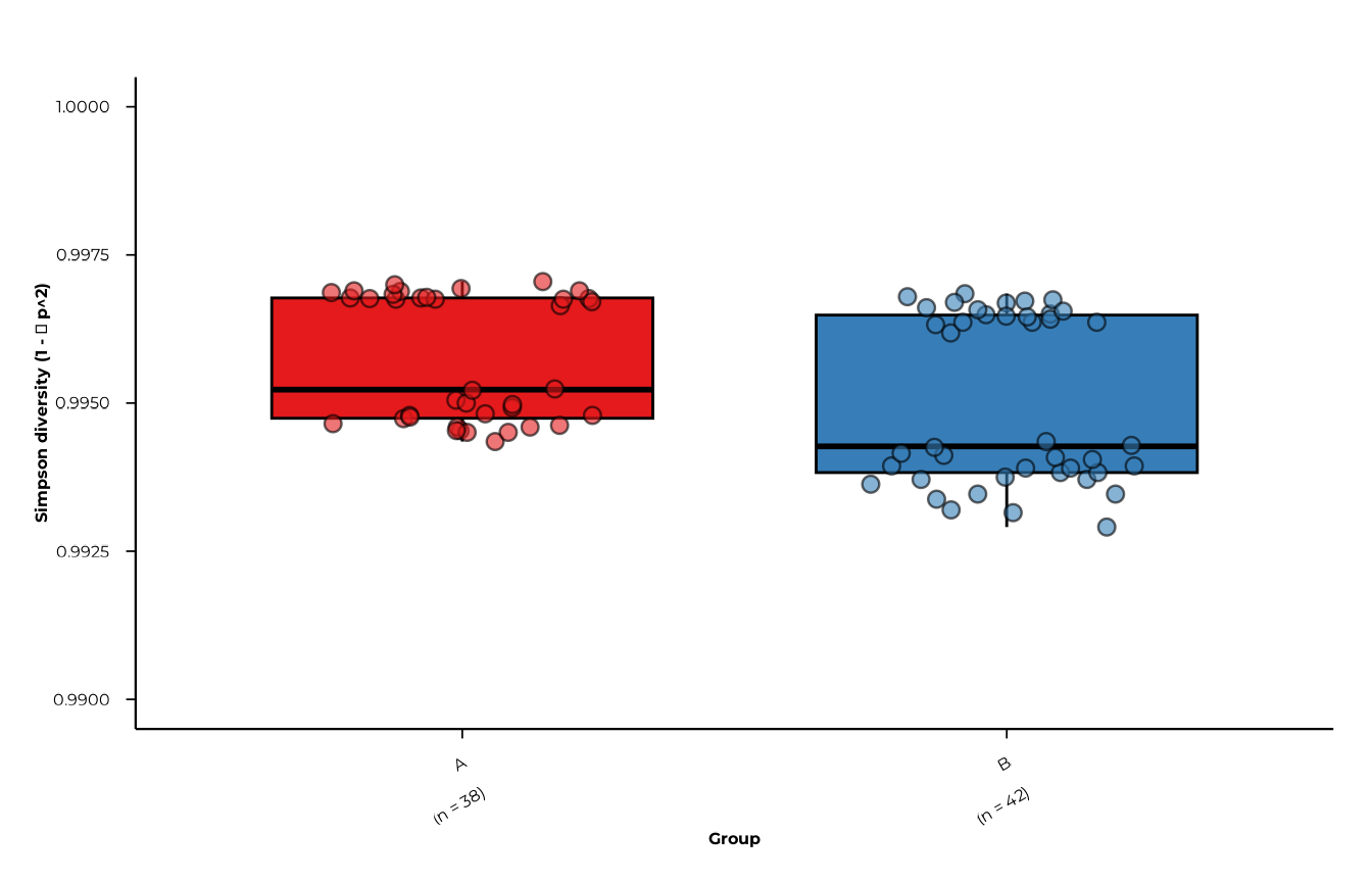
Plotting the interaction table
When group_interaction = TRUE, the interaction element
stores the combined label in a column called
phip_interaction.
plot_alpha(
  alpha_inter,
  metric           = "richness",
  group_col        = "phip_interaction",
  interaction_only = TRUE
)
#> [09:29:55] INFO  plotting alpha diversity (precomputed)
#>                  -> metric: richness
#> [09:29:55] INFO  selected interaction table
#>                    - group * timepoint
#> [09:29:55] OK    plotting alpha diversity (precomputed) - done
#>                  -> elapsed: 0.062s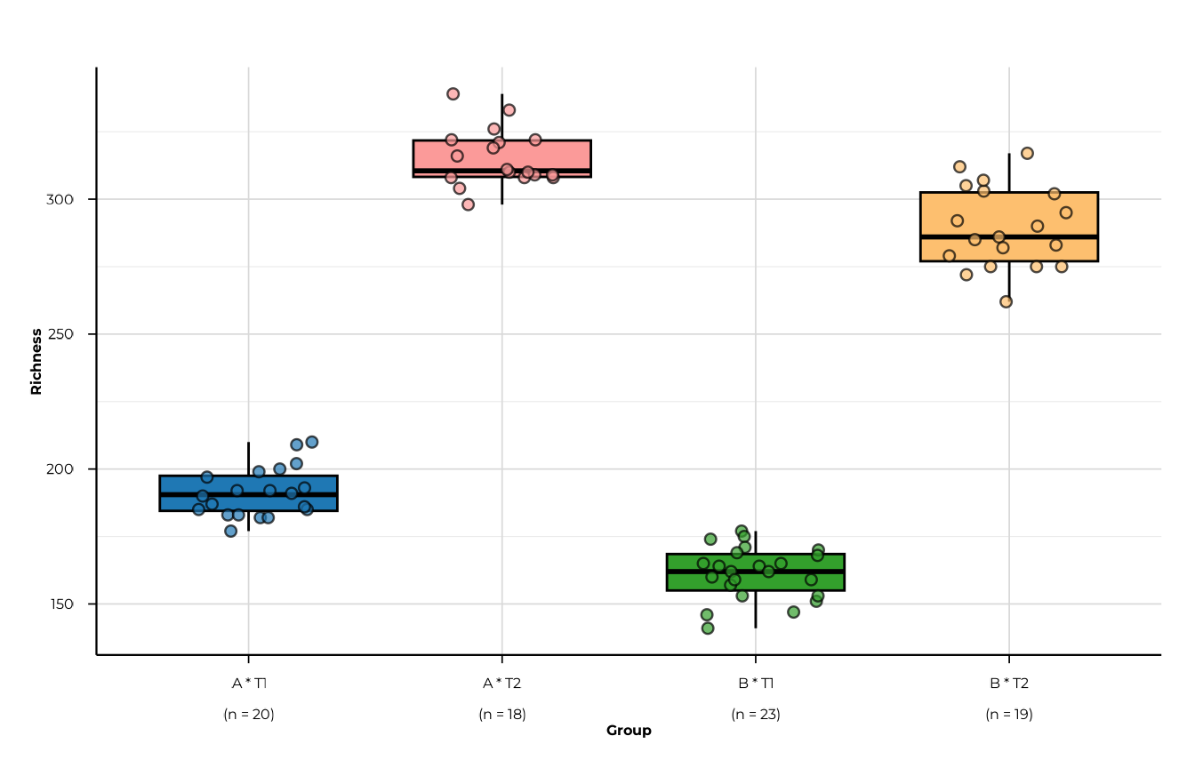
plot_alpha_interactive() — plotly
The interactive version mirrors the static API and returns a plotly widget, making it suitable for HTML reports and Shiny apps.
plot_alpha_interactive(
  alpha_group,
  metric    = "richness",
  group_col = "group"
)
All display parameters — custom_colors,
x_order, y_range, filter_groups,
facet_by_rank — behave identically to the static
version.
Statistical testing
compute_alpha_significance() runs
global and pairwise hypothesis tests
on every (rank, metric) combination in the alpha diversity
result.
Default: Kruskal-Wallis + Wilcoxon
sig <- compute_alpha_significance(
  alpha_group,
  group_col = "group"
)
sig
#> $global
#> # A tibble: 5 × 5
#>   rank       metric                  statistic  p_value test
#>   <chr>      <chr>                       <dbl>    <dbl> <chr>
#> 1 peptide_id richness                     14.2 0.000168 kruskal-wallis
#> 2 peptide_id shannon_diversity            14.2 0.000168 kruskal-wallis
#> 3 peptide_id simpson_diversity            14.2 0.000168 kruskal-wallis
#> 4 peptide_id pielou_evenness             Inf   0        kruskal-wallis
#> 5 peptide_id berger_parker_dominance      14.2 0.000168 kruskal-wallis
#>
#> $pairwise
#> # A tibble: 5 × 9
#>   rank       metric           group1 group2   p_raw   p_adj cohens_d stars test
#>   <chr>      <chr>            <chr>  <chr>    <dbl>   <dbl>    <dbl> <chr> <chr>
#> 1 peptide_id richness         B      A      1.71e-4 1.71e-4   -0.475 ***   wilc…
#> 2 peptide_id shannon_diversi… B      A      1.71e-4 1.71e-4   -0.511 ***   wilc…
#> 3 peptide_id simpson_diversi… B      A      1.71e-4 1.71e-4   -0.563 ***   wilc…
#> 4 peptide_id pielou_evenness  B      A      3.05e-2 3.05e-2    0     *     wilc…
#> 5 peptide_id berger_parker_d… B      A      1.71e-4 1.71e-4    0.563 ***   wilc…
#>
#> attr(,"class")
#> [1] "phip_alpha_significance"
#> attr(,"group_col")
#> [1] "group"
#> attr(,"global_test")
#> [1] "kruskal"
#> attr(,"pairwise_test")
#> [1] "wilcoxon"
#> attr(,"p_adjust_method")
#> [1] "BH"
#> attr(,"metrics")
#> [1] "richness"                "shannon_diversity"
#> [3] "simpson_diversity"       "pielou_evenness"
#> [5] "berger_parker_dominance"
#> attr(,"ranks")
#> [1] "peptide_id"
The return value is a list of class
"phip_alpha_significance" with two tibbles.
Global test
One row per (rank, metric):
sig$global
#> # A tibble: 5 × 5
#>   rank       metric                  statistic  p_value test
#>   <chr>      <chr>                       <dbl>    <dbl> <chr>
#> 1 peptide_id richness                     14.2 0.000168 kruskal-wallis
#> 2 peptide_id shannon_diversity            14.2 0.000168 kruskal-wallis
#> 3 peptide_id simpson_diversity            14.2 0.000168 kruskal-wallis
#> 4 peptide_id pielou_evenness             Inf   0        kruskal-wallis
#> 5 peptide_id berger_parker_dominance      14.2 0.000168 kruskal-wallis
Pairwise comparisons
One row per (rank, metric, pair) with raw and adjusted
p-values, Cohen’s d, and significance stars:
sig$pairwise
#> # A tibble: 5 × 9
#>   rank       metric           group1 group2   p_raw   p_adj cohens_d stars test
#>   <chr>      <chr>            <chr>  <chr>    <dbl>   <dbl>    <dbl> <chr> <chr>
#> 1 peptide_id richness         B      A      1.71e-4 1.71e-4   -0.475 ***   wilc…
#> 2 peptide_id shannon_diversi… B      A      1.71e-4 1.71e-4   -0.511 ***   wilc…
#> 3 peptide_id simpson_diversi… B      A      1.71e-4 1.71e-4   -0.563 ***   wilc…
#> 4 peptide_id pielou_evenness  B      A      3.05e-2 3.05e-2    0     *     wilc…
#> 5 peptide_id berger_parker_d… B      A      1.71e-4 1.71e-4    0.563 ***   wilc…
Choosing the test
sig_anova <- compute_alpha_significance(
  alpha_group,
  group_col     = "group",
  global_test   = "anova",
  pairwise_test = "tukey"
)
sig_anova$global
#> # A tibble: 5 × 5
#>   rank       metric                  statistic p_value test
#>   <chr>      <chr>                       <dbl>   <dbl> <chr>
#> 1 peptide_id richness                     4.50  0.0370 anova
#> 2 peptide_id shannon_diversity            5.21  0.0252 anova
#> 3 peptide_id simpson_diversity            6.32  0.0140 anova
#> 4 peptide_id pielou_evenness              5.79  0.0185 anova
#> 5 peptide_id berger_parker_dominance      6.32  0.0140 anova
p-value adjustment
Any method accepted by p.adjust() is supported:
sig_bonf <- compute_alpha_significance(
  alpha_group,
  group_col       = "group",
  p_adjust_method = "bonferroni"
)
sig_bonf$pairwise[, c("metric", "group1", "group2", "p_raw", "p_adj", "stars")]
#> # A tibble: 5 × 6
#>   metric                  group1 group2    p_raw    p_adj stars
#>   <chr>                   <chr>  <chr>     <dbl>    <dbl> <chr>
#> 1 richness                B      A      0.000171 0.000171 ***
#> 2 shannon_diversity       B      A      0.000171 0.000171 ***
#> 3 simpson_diversity       B      A      0.000171 0.000171 ***
#> 4 pielou_evenness         B      A      0.0305   0.0305   *
#> 5 berger_parker_dominance B      A      0.000171 0.000171 ***
Restricting to a subset of metrics
sig_rich <- compute_alpha_significance(
  alpha_group,
  group_col = "group",
  metric    = c("richness", "shannon_diversity")
)
sig_rich$global
#> # A tibble: 2 × 5
#>   rank       metric            statistic  p_value test
#>   <chr>      <chr>                 <dbl>    <dbl> <chr>
#> 1 peptide_id richness               14.2 0.000168 kruskal-wallis
#> 2 peptide_id shannon_diversity      14.2 0.000168 kruskal-wallis
Multi-rank significance
When alpha was computed at multiple ranks, significance is tested at every rank automatically:
sig_tax <- compute_alpha_significance(
  alpha_tax,
  group_col = "group",
  metric    = "richness"
)
dplyr::select(sig_tax$global, rank, metric, statistic, p_value)
#> # A tibble: 3 × 4
#>   rank       metric   statistic    p_value
#>   <chr>      <chr>        <dbl>      <dbl>
#> 1 peptide_id richness      14.2   0.000168
#> 2 family     richness     NaN   NaN
#> 3 genus      richness     NaN   NaN
Visualising significance
plot_alpha_significance() offers two display modes.
Table mode
Returns the filtered pairwise tibble — useful for including in reports or further processing:
plot_alpha_significance(
  sig,
  metric      = "richness",
  type        = "table",
  p_threshold = 0.05
)
#> # A tibble: 1 × 9
#>   rank       metric   group1 group2    p_raw    p_adj cohens_d stars test
#>   <chr>      <chr>    <chr>  <chr>     <dbl>    <dbl>    <dbl> <chr> <chr>
#> 1 peptide_id richness B      A      0.000171 0.000171   -0.475 ***   wilcoxon
Set p_threshold = 1 to retrieve all pairs regardless of
significance.
plot_alpha_significance(
sig,
metric = "richness",
type = "table",
p_threshold = 1
)
#> # A tibble: 1 × 9
#> rank metric group1 group2 p_raw p_adj cohens_d stars test
#> <chr> <chr> <chr> <chr> <dbl> <dbl> <dbl> <chr> <chr>
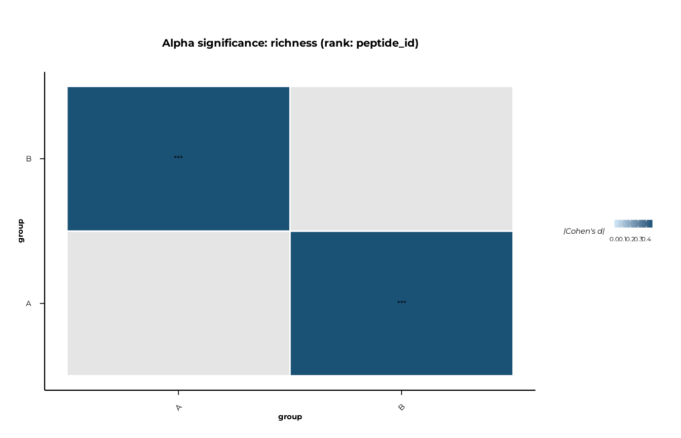
#> 1 peptide_id richness B A 0.000171 0.000171 -0.475 *** wilcoxonHeatmap mode
Produces a Cohen’s d heatmap with significance stars overlaid. Non-significant pairs (p_adj > threshold) are shown in grey.
plot_alpha_significance(
  sig,
  metric      = "richness",
  type        = "heatmap",
  p_threshold = 1     # show all pairs; colour by effect size
)
Heatmap across metrics
Loop over metrics to produce one heatmap per metric:
for (m in attr(sig, "metrics")) {
  print(
    plot_alpha_significance(sig, metric = m, type = "heatmap", p_threshold = 1)
  )
}
Significance brackets on boxplots
Pass a "phip_alpha_significance" object to
plot_alpha() via the significance argument,
and set show_significance = TRUE to overlay pairwise
brackets automatically. The ggsignif package must be
installed.
plot_alpha(
  alpha_group,
  metric            = "richness",
  group_col         = "group",
  significance      = sig,
  show_significance = TRUE,
  sig_p_threshold   = 0.05
)
#> [09:29:57] INFO  plotting alpha diversity (precomputed)
#>                  -> metric: richness
#> [09:29:57] OK    plotting alpha diversity (precomputed) - done
#>                  -> elapsed: 0.111s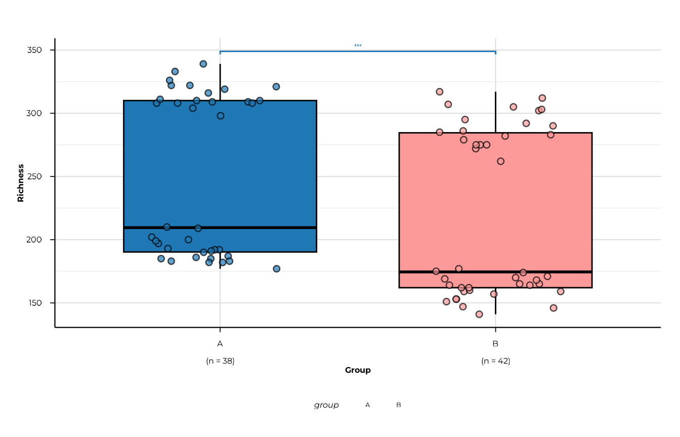
Tune the bracket geometry with sig_step_increase and
sig_tip_length:
plot_alpha(
  alpha_group,
  metric            = "shannon_diversity",
  group_col         = "group",
  significance      = sig,
  show_significance = TRUE,
  sig_p_threshold   = 0.1,
  sig_step_increase = 0.08,
  sig_tip_length    = 0.005
)
#> [09:29:58] INFO  plotting alpha diversity (precomputed)
#>                  -> metric: shannon_diversity
#> [09:29:58] OK    plotting alpha diversity (precomputed) - done
#>                  -> elapsed: 0.108s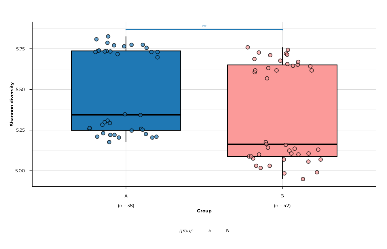
Putting it all together
A typical analysis runs in four steps:
# 1. Compute diversity at peptide and family level
alpha <- compute_alpha(
  pd,
  group_cols        = c("group", "timepoint"),
  ranks             = c("peptide_id", "family"),
  group_interaction = TRUE
)

# 2. Visualise
plot_alpha(alpha, metric = "richness",    group_col = "group")
plot_alpha(alpha, metric = "pielou_evenness", group_col = "timepoint",
                     x_order = c("T1", "T2"),
                     x_labels = c(T1 = "Baseline", T2 = "Follow-up"))

# 3. Test
sig <- compute_alpha_significance(alpha, group_col = "group")

# 4. Report
sig$global
plot_alpha_significance(sig, type = "heatmap", p_threshold = 1)
plot_alpha(alpha, metric = "richness", group_col = "group",
                     significance = sig, show_significance = TRUE)
Session info
sessionInfo()
#> R version 4.6.1 (2026-06-24)
#> Platform: x86_64-pc-linux-gnu
#> Running under: Ubuntu 24.04.4 LTS
#>
#> Matrix products: default
#> BLAS:   /usr/lib/x86_64-linux-gnu/openblas-pthread/libblas.so.3
#> LAPACK: /usr/lib/x86_64-linux-gnu/openblas-pthread/libopenblasp-r0.3.26.so;  LAPACK version 3.12.0
#>
#> locale:
#>  [1] LC_CTYPE=C.UTF-8       LC_NUMERIC=C           LC_TIME=C.UTF-8
#>  [4] LC_COLLATE=C.UTF-8     LC_MONETARY=C.UTF-8    LC_MESSAGES=C.UTF-8
#>  [7] LC_PAPER=C.UTF-8       LC_NAME=C              LC_ADDRESS=C
#> [10] LC_TELEPHONE=C         LC_MEASUREMENT=C.UTF-8 LC_IDENTIFICATION=C
#>
#> time zone: UTC
#> tzcode source: system (glibc)
#>
#> attached base packages:
#> [1] stats     graphics  grDevices utils     datasets  methods   base
#>
#> other attached packages:
#> [1] phiper_0.4.3
#>
#> loaded via a namespace (and not attached):
#>  [1] tidyr_1.3.2           utf8_1.2.6            sass_0.4.10
#>  [4] generics_0.1.4        digest_0.6.39         magrittr_2.0.5
#>  [7] evaluate_1.0.5        grid_4.6.1            RColorBrewer_1.1-3
#> [10] sysfonts_0.8.9        showtextdb_3.0        blob_1.3.0
#> [13] fastmap_1.2.0         jsonlite_2.0.0        DBI_1.3.0
#> [16] purrr_1.2.2           scales_1.4.0          textshaping_1.0.5
#> [19] jquerylib_0.1.4       duckdb_1.5.4.3        cli_3.6.6
#> [22] rlang_1.3.0           chk_0.10.0            dbplyr_2.6.0
#> [25] phiperio_0.5.2        withr_3.0.3           cachem_1.1.0
#> [28] yaml_2.3.12           otel_0.2.0            tools_4.6.1
#> [31] ggsignif_0.6.4        dplyr_1.2.1           ggplot2_4.0.3
#> [34] showtext_0.9-8        vctrs_0.7.3           R6_2.6.1
#> [37] lifecycle_1.0.5       fs_2.1.0              htmlwidgets_1.6.4
#> [40] ragg_1.5.2            pkgconfig_2.0.3       desc_1.4.3
#> [43] pkgdown_2.2.1         RcppParallel_5.1.11-2 pillar_1.11.1
#> [46] bslib_0.11.0          gtable_0.3.6          glue_1.8.1
#> [49] Rcpp_1.1.2            systemfonts_1.3.2     xfun_0.60
#> [52] tibble_3.3.1          tidyselect_1.2.1      knitr_1.51
#> [55] farver_2.1.2          htmltools_0.5.9       labeling_0.4.3
#> [58] rmarkdown_2.31        compiler_4.6.1        S7_0.2.2