Prevalence of Presence (POP) Analysis in PhIP-seq

Overview

POP (Prevalence Of Presence) measures how often each feature is detected across the samples in a group. For each (rank, feature, group pair) the analysis asks: does the fraction of samples carrying this feature differ between the two groups?

This vignette walks through the complete POP workflow in phiper:

Computing prevalence and p-values with compute_pop()
Visualising results as scatter plots with scatter_static() and scatter_interactive()
Volcano plots with volcano_static() and volcano_interactive()

Setup

library(phiper)

Load the bundled example dataset. It contains two patient groups (A, B) measured at two timepoints (T1, T2) across 1 000 simulated peptides.

pd <- load_example_data()
#> [17:16:19] INFO  Constructing <phip_data> object
#>                  -> create_data()
#> [17:16:19] INFO  Fetching peptide metadata library via get_peptide_library()
#>                    - libraries: combined
#> [17:16:19] INFO  Retrieving peptide metadata into DuckDB cache
#>                  -> get_peptide_library(library = combined, force_refresh =
#>                     FALSE)
#> [17:16:19] INFO  Opened DuckDB connection
#>                    - cache dir:
#>                      /home/runner/.cache/R/phiperio/peptide_meta/phip_cache.duckdb
#>                    - tables: peptide_meta_combined
#> [17:16:19] OK    Using cached peptide_meta_combined (fast path)
#> [17:16:19] OK    Retrieving peptide metadata into DuckDB cache - done
#>                  -> elapsed: 0.046s
#> [17:16:19] OK    Peptide metadata acquired
#> [17:16:19] INFO  Validating <phip_data>
#>                  -> validate_phip_data()
#> [17:16:19] INFO  Checking structural requirements (shape & mandatory columns)
#> [17:16:19] INFO  Checking outcome family availability (exist / fold_change /
#>                  raw_counts)
#> [17:16:19] INFO  Checking collisions with reserved names
#>                    - subject_id, sample_id, timepoint, peptide_id, exist,
#>                      fold_change, counts_input, counts_hit
#> [17:16:19] INFO  Ensuring all columns are atomic (no list-cols)
#> [17:16:19] INFO  Checking key uniqueness
#> [17:16:19] INFO  Validating value ranges & types for outcomes
#> [17:16:19] INFO  Assessing sparsity (NA/zero prevalence vs threshold)
#>                    - warn threshold: 50%
#> [17:16:19] INFO  Checking peptide_id coverage against peptide_library
#> [17:16:20] INFO  Checking full grid completeness (peptide * sample)
#> [17:16:20] INFO  Counts table is not a full peptide * sample grid
#>                    - observed rows: 78200
#>                    - expected rows: 156000
#> [17:16:20] OK    Validating <phip_data> - done
#>                  -> elapsed: 0.461s
#> [17:16:20] OK    Constructing <phip_data> object - done
#>                  -> elapsed: 0.553s
pd
#> ── <phip_data> ───────────────────────────────────────────────────────────────── 
#> 
#> counts (first 5 rows): 
#> # A tibble: 5 × 9
#>   sample_id subject_id group timepoint peptide_id     exist counts_control
#>   <chr>     <chr>      <chr> <chr>     <chr>          <int>          <int>
#> 1 B_T1_1    1          B     T1        agilent_100642     0             16
#> 2 B_T1_1    1          B     T1        agilent_100997     1             18
#> 3 B_T1_1    1          B     T1        agilent_10133      0             15
#> 4 B_T1_1    1          B     T1        agilent_101516     0             29
#> 5 B_T1_1    1          B     T1        agilent_101615     0             16
#> # ℹ 2 more variables: counts_hits <int>, fold_change <dbl>
#> 
#> table size: 78,200 rows x 9 columns
#> 
#> peptide library preview (first 5 rows): 
#> # A tibble: 5 × 8
#>   peptide_id    Fullname                 species genus family order class common
#>   <chr>         <chr>                    <chr>   <chr> <chr>  <chr> <chr> <chr> 
#> 1 agilent_1     Chromodomain-helicase-D… Homo s… Homo  Homin… Prim… Mamm… Human 
#> 2 agilent_10    Lipase 2 precursor (Gly… Staphy… Stap… Staph… Baci… Baci… NA    
#> 3 agilent_100   cell surface protein pr… Porphy… Porp… Porph… Bact… Bact… NA    
#> 4 agilent_1000  Coagulation factor VIII… Homo s… Homo  Homin… Prim… Mamm… Human 
#> 5 agilent_10000 transmembrane serine/th… Mycoba… Myco… Mycob… Myco… Acti… NA    
#> ... plus 37 more columns
#> 
#> library size: 357,190 rows x 45 columns
#> 
#> meta flags: 
#>   con:            <duckdb_connection>
#>   peptide_libraries: combined
#>   longitudinal:   TRUE
#>   exist:          TRUE
#>   fold_change:    TRUE
#>   raw_counts:     FALSE
#>   extra_cols:     group, counts_control, counts_hits
#>   peptide_con:    <duckdb_connection>
#>   materialise_table: TRUE
#>   finalizer_env:  <environment>
#>   full_cross:     FALSE

Note. The example data are entirely simulated and have no biological meaning. They exist solely to demonstrate the API.

Computing prevalence: `compute_pop()`

Unpaired design — group comparison

The workhorse function is compute_pop(). Supply a phip_data object, the rank(s) at which prevalence should be aggregated, and the binary grouping column(s).

pop_group <- compute_pop(
  pd,
  rank_cols  = "peptide_id",
  group_cols = "group"
)
#> [17:16:20] INFO  compute_pop
#> [17:16:20] INFO  compute_pop
#>                    - ranks : peptide_id
#>                    - group_cols: group
#>                    - exist_col : exist
#>                    - pop_k_min : 1
#>                    - paired : FALSE
#> [17:16:20] INFO  ranks resolved
#>                    - available: peptide_id
#> [17:16:20] INFO  computing cohort sizes and validating binary group_cols
#> [17:16:20] INFO  computing presence per sample via k-of-n rule
#> [17:16:20] INFO  counting present samples per feature (pop, unpaired)
#> [17:16:20] INFO  building pairwise comparisons
#> [17:16:22] OK    materialized; computing Fisher p-values
#>                    - table: ph_pop_20261006_171620
#> [17:16:22] OK    done (compute_pop, unpaired)
#>                    - rows : 1950
#>                    - ranks : peptide_id
#>                    - k_min : 1
#> [17:16:22] OK    compute_pop - done
#>                  -> elapsed: 2.53s

The result is a plain data.frame with one row per (rank, feature, group pair):

head(pop_group)
#>         rank        feature group_col group1 n1 N1 prop1 percent1 group2 n2 N2
#> 1 peptide_id agilent_100642     group      A  0 38     0        0      B  8 42
#> 2 peptide_id agilent_100997     group      A  0 38     0        0      B  6 42
#> 3 peptide_id  agilent_10133     group      A  0 38     0        0      B  5 42
#> 4 peptide_id agilent_101516     group      A  0 38     0        0      B 17 42
#> 5 peptide_id agilent_101615     group      A  0 38     0        0      B  9 42
#> 6 peptide_id agilent_101998     group      A  0 38     0        0      B 11 42
#>       prop2 percent2      ratio delta_ratio        p_raw n_peptides
#> 1 0.1904762 19.04762 0.06907895   -6.238095 5.758809e-03          1
#> 2 0.1428571 14.28571 0.09210526   -4.428571 2.664380e-02          1
#> 3 0.1190476 11.90476 0.11052632   -3.523810 5.626494e-02          1
#> 4 0.4047619 40.47619 0.03250774  -14.380952 2.792824e-06          1
#> 5 0.2142857 21.42857 0.06140351   -7.142857 2.625712e-03          1
#> 6 0.2619048 26.19048 0.05023923   -8.952381 5.233874e-04          1

What’s in the output?

Column	Description
`rank`	Rank at which the feature is defined (e.g. `"peptide_id"`)
`feature`	Feature identifier
`group_col`	Name of the grouping column
`group1`, `group2`	The two group labels being compared
`n1`, `N1`	Positives and total samples in group 1
`prop1`, `percent1`	Prevalence in group 1 (proportion and percentage)
`n2`, `N2`	Positives and total samples in group 2
`prop2`, `percent2`	Prevalence in group 2
`ratio`	`prop1 / prop2` (with small-sample epsilon correction)
`delta_ratio`	Signed fold-change: `prop1/prop2 − 1` (or its negative)
`p_raw`	Fisher’s exact test p-value (unpaired)
`n_peptides`	Number of peptides contributing to this feature

names(pop_group)
#>  [1] "rank"        "feature"     "group_col"   "group1"      "n1"         
#>  [6] "N1"          "prop1"       "percent1"    "group2"      "n2"         
#> [11] "N2"          "prop2"       "percent2"    "ratio"       "delta_ratio"
#> [16] "p_raw"       "n_peptides"
nrow(pop_group)
#> [1] 1950

Multiple group columns

Pass a character vector to group_cols to test several grouping variables in one call.

pop_multi <- compute_pop(
  pd,
  rank_cols  = "peptide_id",
  group_cols = c("group", "timepoint")
)
#> [17:16:22] INFO  compute_pop
#> [17:16:22] INFO  compute_pop
#>                    - ranks : peptide_id
#>                    - group_cols: group, timepoint
#>                    - exist_col : exist
#>                    - pop_k_min : 1
#>                    - paired : FALSE
#> [17:16:22] INFO  ranks resolved
#>                    - available: peptide_id
#> [17:16:23] INFO  computing cohort sizes and validating binary group_cols
#> [17:16:23] INFO  computing presence per sample via k-of-n rule
#> [17:16:23] INFO  counting present samples per feature (pop, unpaired)
#> [17:16:23] INFO  building pairwise comparisons
#> [17:16:25] OK    materialized; computing Fisher p-values
#>                    - table: ph_pop_20261006_171623
#> [17:16:27] OK    done (compute_pop, unpaired)
#>                    - rows : 3900
#>                    - ranks : peptide_id
#>                    - k_min : 1
#> [17:16:27] OK    compute_pop - done
#>                  -> elapsed: 4.183s

# One block of rows per group column
table(pop_multi$group_col)
#> 
#>     group timepoint 
#>      1950      1950

Multiple ranks

rank_cols accepts any column present in the peptide library. Pass "peptide_id" for peptide-level results, or taxonomic rank columns (e.g. "family", "genus") for higher-level aggregation.

Note on this toy example. The synthetic peptides do not map to real library annotations, so all higher-rank columns are empty. In a real PhIP-seq experiment, family- and genus-level rows reflect the taxonomic breadth of each patient’s reactivity.

pop_tax <- compute_pop(
  pd,
  rank_cols  = c("peptide_id", "family", "genus"),
  group_cols = "group"
)
table(pop_tax$rank)

k-of-n presence threshold

By default a sample is called positive for a feature if at least one of its contributing peptides is present (pop_k_min = 1). Raise this threshold to require, say, at least two peptides before calling a sample positive — useful for filtering out singleton hits.

pop_k2 <- compute_pop(
  pd,
  rank_cols  = "peptide_id",
  group_cols = "group",
  pop_k_min  = 2L
)
#> [17:16:27] INFO  compute_pop
#> [17:16:27] INFO  compute_pop
#>                    - ranks : peptide_id
#>                    - group_cols: group
#>                    - exist_col : exist
#>                    - pop_k_min : 2
#>                    - paired : FALSE
#> [17:16:27] INFO  ranks resolved
#>                    - available: peptide_id
#> [17:16:27] INFO  computing cohort sizes and validating binary group_cols
#> [17:16:27] INFO  computing presence per sample via k-of-n rule
#> [17:16:27] INFO  counting present samples per feature (pop, unpaired)
#> [17:16:27] INFO  building pairwise comparisons
#> [17:16:29] OK    materialized; computing Fisher p-values
#>                    - table: ph_pop_20261006_171627
#> [17:16:29] OK    done (compute_pop, unpaired)
#>                    - rows : 0
#>                    - ranks :
#>                    - k_min : 2
#> [17:16:29] OK    compute_pop - done
#>                  -> elapsed: 2.013s

# Higher k_min → fewer positives
mean(pop_k2$n1) < mean(pop_group$n1)
#> [1] NA

Paired design — timepoint comparison

When the same subjects are measured at two timepoints, the paired design uses McNemar’s exact binomial test instead of Fisher’s exact test, which is more powerful because it accounts for within-subject correlation.

Set paired to the name of the column that links samples from the same subject across timepoints.

pop_paired <- compute_pop(
  pd,
  rank_cols  = "peptide_id",
  group_cols = "timepoint",
  paired     = "subject_id"
)
#> [17:16:29] INFO  compute_pop
#> [17:16:29] INFO  compute_pop
#>                    - ranks : peptide_id
#>                    - group_cols: timepoint
#>                    - exist_col : exist
#>                    - pop_k_min : 1
#>                    - paired : subject_id
#> [17:16:29] INFO  ranks resolved
#>                    - available: peptide_id
#> [17:16:29] INFO  computing cohort sizes and validating binary group_cols
#> [17:16:29] INFO  computing presence per sample via k-of-n rule
#> [17:16:29] INFO  paired design: running McNemar exact (binomial)
#> [17:16:31] OK    done (compute_pop, paired)
#>                    - rows : 1950
#>                    - ranks : peptide_id
#>                    - k_min : 1
#> [17:16:31] OK    compute_pop - done
#>                  -> elapsed: 2.023s

head(pop_paired)
#>         rank        feature group_col group1 n1 N1      prop1  percent1 group2
#> 1 peptide_id agilent_100642 timepoint     T1  2 19 0.10526316 10.526316     T2
#> 2 peptide_id agilent_100997 timepoint     T1  2 19 0.10526316 10.526316     T2
#> 3 peptide_id  agilent_10133 timepoint     T1  1 19 0.05263158  5.263158     T2
#> 4 peptide_id agilent_101516 timepoint     T1  6 19 0.31578947 31.578947     T2
#> 5 peptide_id agilent_101615 timepoint     T1  1 19 0.05263158  5.263158     T2
#> 6 peptide_id agilent_101998 timepoint     T1  3 19 0.15789474 15.789474     T2
#>   n2 N2     prop2 percent2    p_raw n_peptides
#> 1  6 19 0.3157895 31.57895 0.125000          1
#> 2  4 19 0.2105263 21.05263 0.625000          1
#> 3  4 19 0.2105263 21.05263 0.250000          1
#> 4  8 19 0.4210526 42.10526 0.687500          1
#> 5  8 19 0.4210526 42.10526 0.015625          1
#> 6  6 19 0.3157895 31.57895 0.250000          1

The paired output does not include ratio or delta_ratio — the test statistic is the McNemar discordant-pair ratio, which is reflected in p_raw.

names(pop_paired)
#>  [1] "rank"       "feature"    "group_col"  "group1"     "n1"        
#>  [6] "N1"         "prop1"      "percent1"   "group2"     "n2"        
#> [11] "N2"         "prop2"      "percent2"   "p_raw"      "n_peptides"

Scatter plots

Scatter plots compare the prevalence of every feature in group 1 (x-axis) against group 2 (y-axis). Points on the diagonal represent features with equal prevalence across groups; deviations indicate differential carriage.

`scatter_static()` — ggplot2

The simplest call takes the compute_pop() result directly. Coloring is determined automatically from BH-corrected p-values: "significant (BH)", "nominal only", "not significant".

scatter_static(pop_group)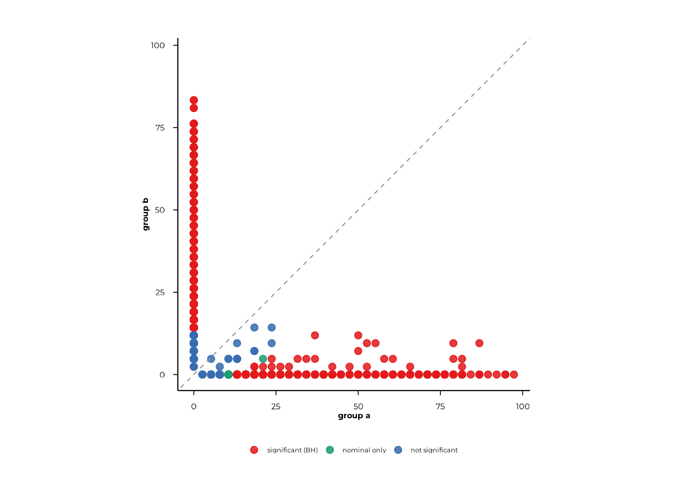

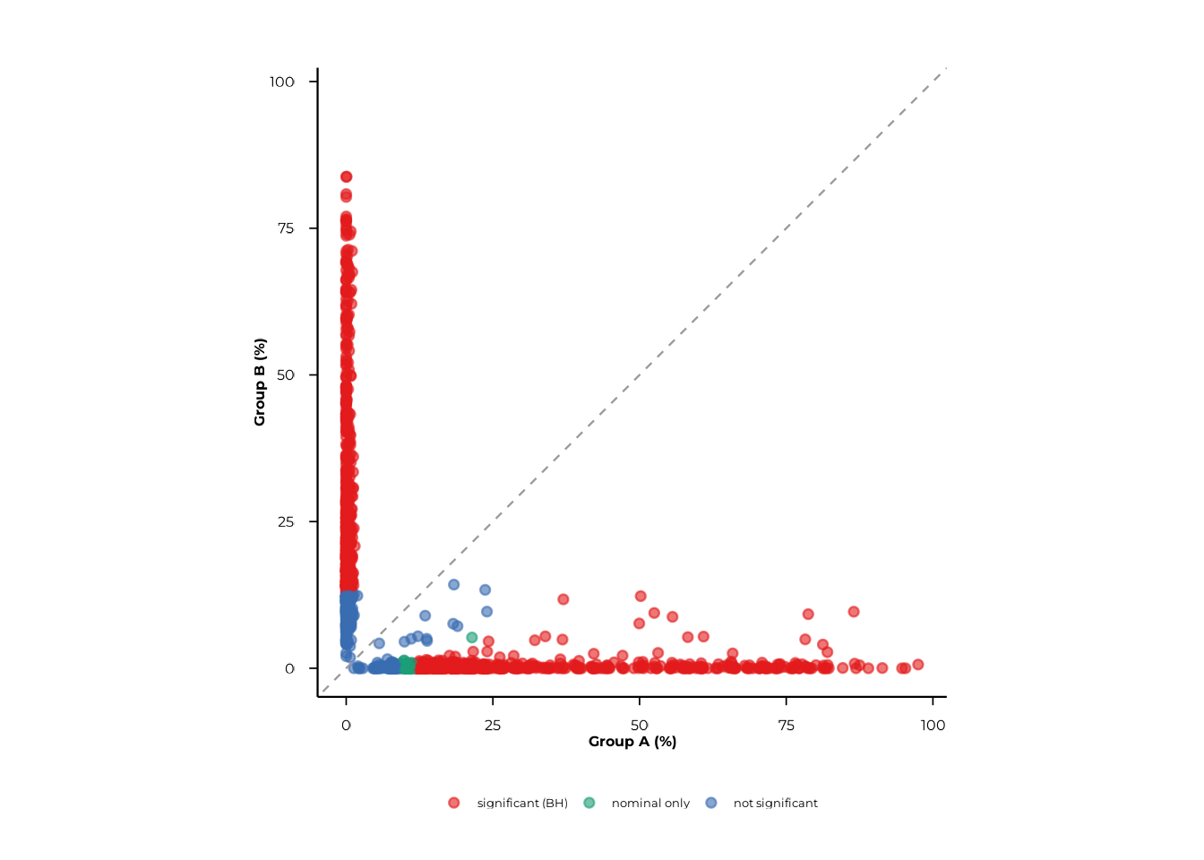
Use pair to restrict the plot to a specific group contrast and xlab/ylab to label the axes.

scatter_static(
  pop_group,
  pair  = c("A", "B"),
  xlab  = "Group A (%)",
  ylab  = "Group B (%)",
  alpha = 0.05
)

Pass rank to display a single rank when the result contains multiple ranks.

scatter_static(pop_tax, rank = "family", pair = c("A", "B"))

Graphical parameters are passed via ...:

Parameter	Default	Effect
`point_size`	2	Point diameter
`point_alpha`	0.85	Point opacity
`jitter_width_pp`	0	Horizontal jitter (percentage points)
`jitter_height_pp`	0	Vertical jitter (percentage points)
`font_size`	12	Base font size

scatter_static(
  pop_group,
  pair             = c("A", "B"),
  xlab             = "Group A (%)",
  ylab             = "Group B (%)",
  point_size       = 1.5,
  point_alpha      = 0.6,
  jitter_width_pp  = 0.5,
  jitter_height_pp = 0.5
)

color_by — scatter_static() also accepts a color_by named vector (e.g. c("species" = "Staphylococcus aureus")) to highlight points by peptide-library metadata. This requires a real peptide library with matching annotations and is not demonstrated here.

`scatter_interactive()` — plotly

The interactive version mirrors the static API and returns a plotly widget suitable for HTML reports and Shiny dashboards. Hovering over a point shows its feature identifier, raw counts, prevalence percentages, and p-values.

scatter_interactive(
  pop_group,
  pair  = c("A", "B"),
  xlab  = "Group A (%)",
  ylab  = "Group B (%)",
  alpha = 0.05
)

An optional background_df argument lets you overlay a second set of points (e.g. all peptides from a different comparison) as a grey reference layer:

scatter_interactive(
  pop_group,
  pair            = c("A", "B"),
  background_df   = pop_multi[pop_multi$group_col == "timepoint", ],
  show_background = TRUE,
  background_name = "timepoint background"
)

Volcano plots

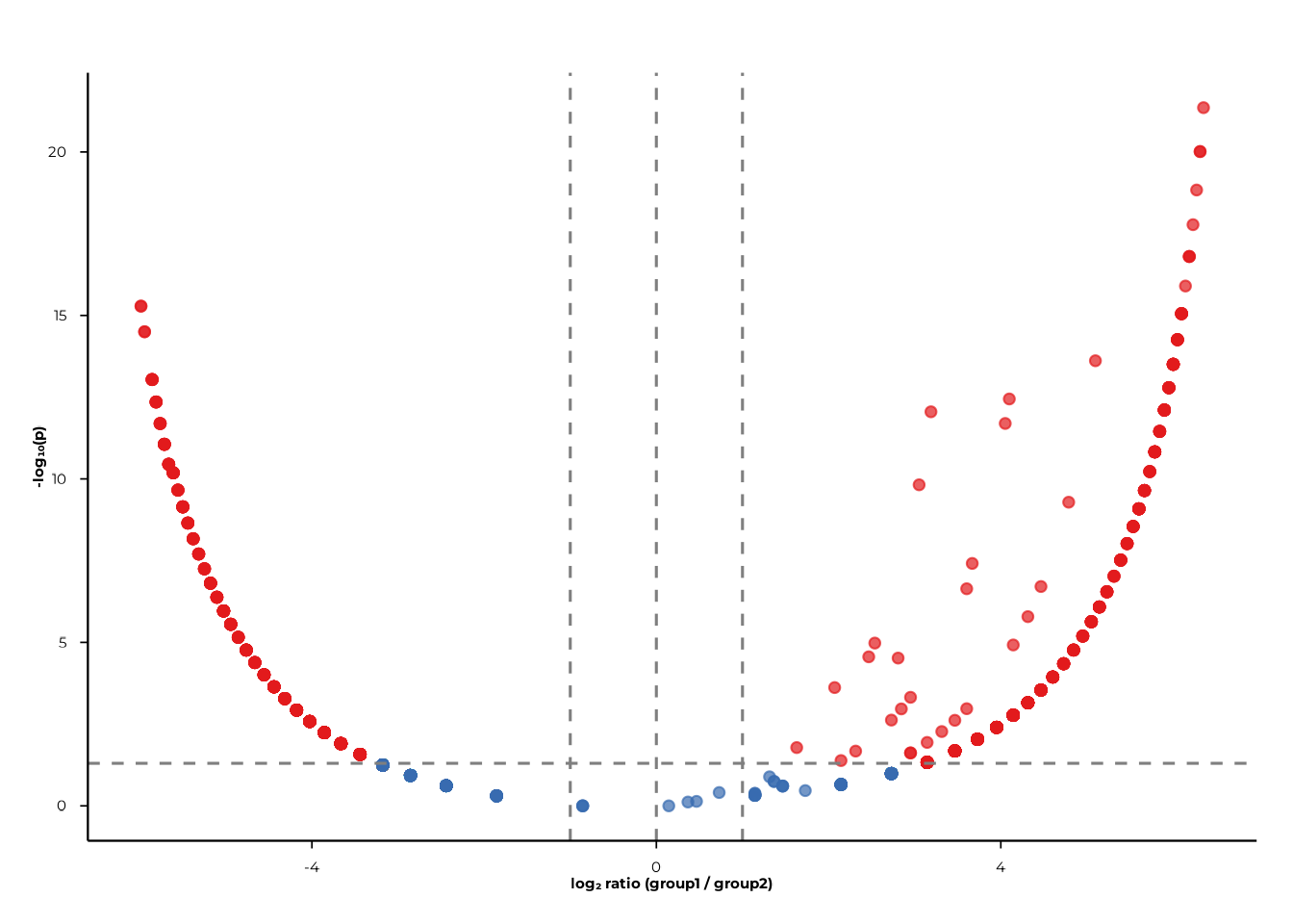
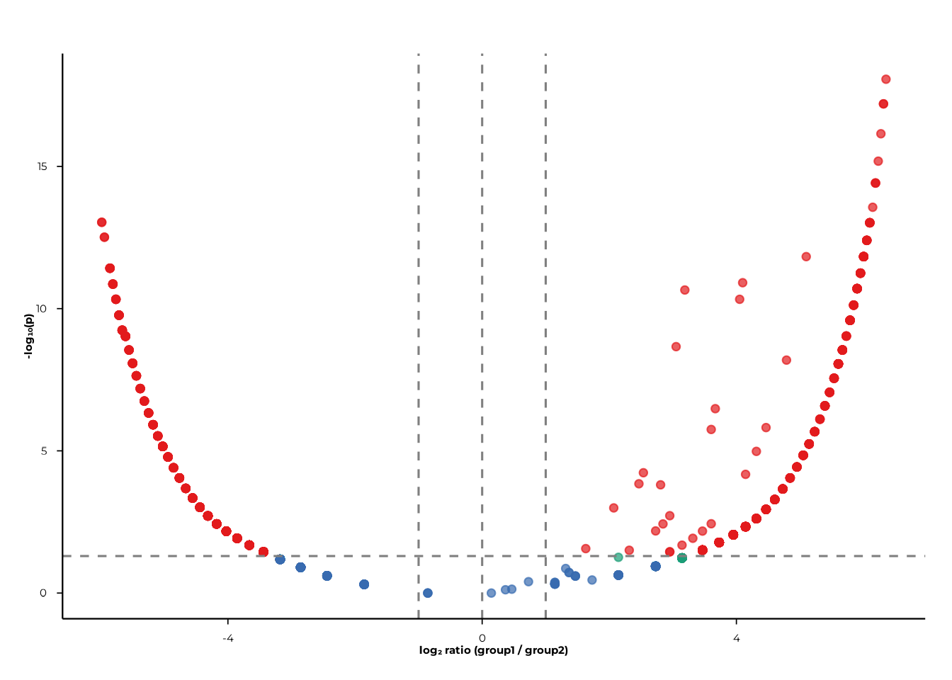
Volcano plots display log₂ ratio (x-axis) against −log₁₀(p) (y-axis), making it easy to spot features with both large effect sizes and small p-values.

`volcano_static()` — ggplot2

volcano_static(pop_group)

Filter to a specific contrast and rank with pair and rank:

volcano_static(
  pop_group,
  pair = c("A", "B"),
  rank = "peptide_id"
)

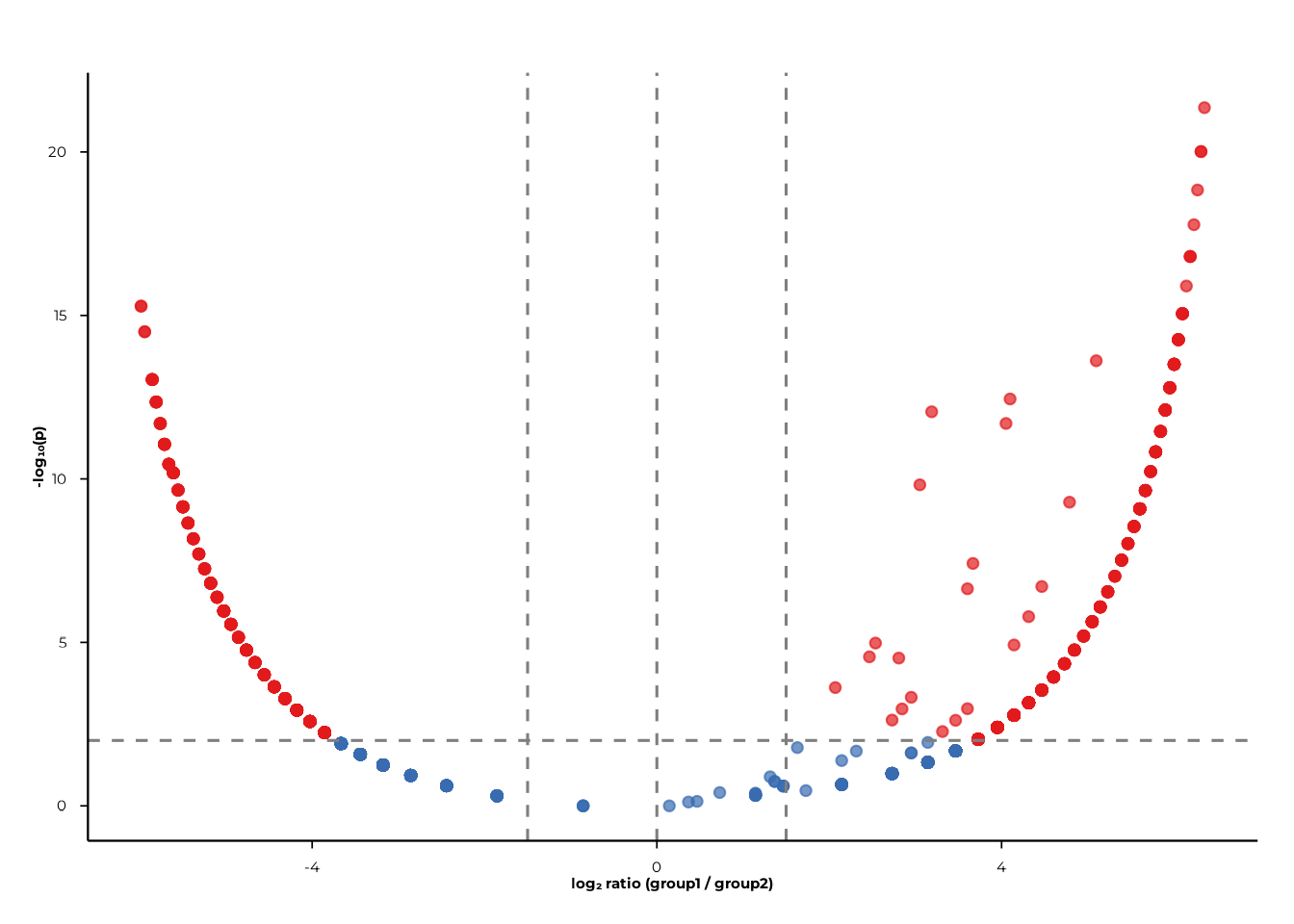
Cutoffs

fc_cut (absolute log₂ fold-change) and p_cut (p-value) control where the dashed reference lines are drawn and how significance categories are assigned.

volcano_static(
  pop_group,
  pair   = c("A", "B"),
  fc_cut = 1.5,
  p_cut  = 0.01
)

BH correction

Set p_mode = "bh" to apply Benjamini–Hochberg correction per-plot. The y-axis then displays −log₁₀(p_BH).

volcano_static(
  pop_group,
  pair   = c("A", "B"),
  p_mode = "bh",
  p_cut  = 0.05
)

color_by — like the scatter plots, volcano_static() accepts a color_by argument to highlight features by peptide-library metadata. This requires real library annotations and is not demonstrated here.

`volcano_interactive()` — plotly

volcano_interactive(
  pop_group,
  pair   = c("A", "B"),
  p_mode = "bh",
  p_cut  = 0.05,
  fc_cut = 1
)

Hovering over a point shows the feature identifier, rank, group labels, log₂ ratio, and −log₁₀(p).

Putting it all together

A typical POP analysis runs in three steps:

# 1. Compute prevalence
pop <- compute_pop(
  pd,
  rank_cols  = c("peptide_id", "family"),
  group_cols = "group"
)

# Optional paired comparison across timepoints
pop_paired <- compute_pop(
  pd,
  rank_cols  = "peptide_id",
  group_cols = "timepoint",
  paired     = "subject_id"
)

# 2. Scatter: prevalence in group A vs group B
scatter_static(pop, pair = c("A", "B"), xlab = "Group A (%)", ylab = "Group B (%)")
scatter_interactive(pop, pair = c("A", "B"), xlab = "Group A (%)", ylab = "Group B (%)")

# 3. Volcano: effect size and significance
volcano_static(pop,       pair = c("A", "B"), p_mode = "bh")
volcano_interactive(pop,  pair = c("A", "B"), p_mode = "bh")

Session info

sessionInfo()
#> R version 4.6.1 (2026-06-24)
#> Platform: x86_64-pc-linux-gnu
#> Running under: Ubuntu 24.04.5 LTS
#> 
#> Matrix products: default
#> BLAS:   /usr/lib/x86_64-linux-gnu/openblas-pthread/libblas.so.3 
#> LAPACK: /usr/lib/x86_64-linux-gnu/openblas-pthread/libopenblasp-r0.3.26.so;  LAPACK version 3.12.0
#> 
#> locale:
#>  [1] LC_CTYPE=C.UTF-8       LC_NUMERIC=C           LC_TIME=C.UTF-8       
#>  [4] LC_COLLATE=C.UTF-8     LC_MONETARY=C.UTF-8    LC_MESSAGES=C.UTF-8   
#>  [7] LC_PAPER=C.UTF-8       LC_NAME=C              LC_ADDRESS=C          
#> [10] LC_TELEPHONE=C         LC_MEASUREMENT=C.UTF-8 LC_IDENTIFICATION=C   
#> 
#> time zone: UTC
#> tzcode source: system (glibc)
#> 
#> attached base packages:
#> [1] stats     graphics  grDevices utils     datasets  methods   base     
#> 
#> other attached packages:
#> [1] phiper_0.4.14
#> 
#> loaded via a namespace (and not attached):
#>  [1] sass_0.4.10         utf8_1.2.6          future_1.76.0      
#>  [4] generics_0.1.4      tidyr_1.3.2         listenv_1.1.0      
#>  [7] digest_0.6.39       magrittr_2.0.5      evaluate_1.0.5     
#> [10] grid_4.6.1          RColorBrewer_1.1-3  fastmap_1.2.0      
#> [13] blob_1.3.0          jsonlite_2.0.0      DBI_1.3.0          
#> [16] purrr_1.2.2         scales_1.4.0        codetools_0.2-20   
#> [19] textshaping_1.0.5   jquerylib_0.1.4     duckdb_1.5.6       
#> [22] cli_3.6.6           rlang_1.3.0         chk_0.11.0         
#> [25] dbplyr_2.6.0        phiperio_0.6.1      future.apply_1.20.2
#> [28] parallelly_1.48.0   withr_3.0.3         cachem_1.1.0       
#> [31] yaml_2.3.12         otel_0.2.0          parallel_4.6.1     
#> [34] tools_4.6.1         dplyr_1.2.1         ggplot2_4.0.3      
#> [37] globals_0.19.1      vctrs_0.7.3         R6_2.6.1           
#> [40] lifecycle_1.0.5     fs_2.1.0            htmlwidgets_1.6.4  
#> [43] ragg_1.5.2          pkgconfig_2.0.3     desc_1.4.3         
#> [46] pkgdown_2.2.1       RcppParallel_6.2.1  pillar_1.11.1      
#> [49] bslib_0.12.0        gtable_0.3.6        glue_1.8.1         
#> [52] Rcpp_1.1.2          systemfonts_1.3.2   xfun_0.61          
#> [55] tibble_3.3.1        tidyselect_1.2.1    knitr_1.52         
#> [58] farver_2.1.2        htmltools_0.5.9     labeling_0.4.3     
#> [61] rmarkdown_2.32      compiler_4.6.1      S7_0.2.2